Bivariate mapping is an important mapping technique in cartography. Given a set of geographic features, it maps two variables on a single map by combining two different sets of graphic symbols. However, few desktop GIS software packages, including ArcView GIS, provide functions for bivariate mapping. An avenue script named "Bivarleg.ave", intended for bivariate mapping and downloadable from Esri’s web site, merely displays one variable with two sets of symbols. This article introduces a creative way to produce bivariate maps for point, line features and bivariate choropleth maps for polygon features. It is has been successfully implemented in a complex Avenue script.
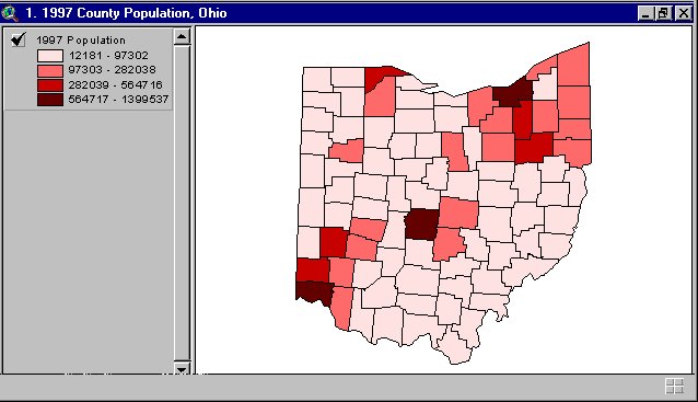
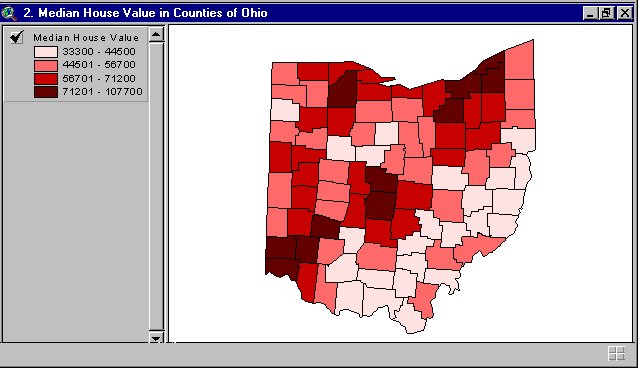
Thematic maps typically represent a single variable using various graphic symbols. Figures 1 and 2 are two thematic maps produced in ArcView GIS. Figure 1 shows the 1997 county population of Ohio. Figure 2 displays the distribution of county-level median house value of Ohio. Both maps have four classes created by natural break classification method. The right panel of the figure displays the map itself; the left panel displays the legend of the map.
Unlike typical thematic maps, a bivariate map displays two variables on the same map. A broad definition of bivariate maps includes all maps that display two variables. Bivariate maps may consist of point features, line features or polygon features.
In conventional cartography, the term "bivariate maps" specifically refers to bivariate choropleth maps that display two variables using graduated color symbols. Since choropleth mapping technique is designed for polygon features, bivariate choropleth maps can not be applied to point and line features.
As a desktop GIS, ArcView is designed to map and visualize a single variable at a time. Although creative use of the functions provided in the default graphic user interface (GUI) can facilitate in generating some types of bivariate maps, it is impossible to generate bivariate choropleth maps without using complex algorithm implemented in Avenue scripts.
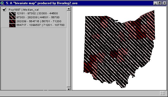
Previous attempts in developing such scripts have failed. The scripts "bivarleg.ave" and "bivarleg2.ave" from the Esri web site are not capable of producing bivariate choropleth maps. They merely display the classification of one variable on the map panel (Figure 3). The display of class intervals of the second variable in the left panel only adds more confusion.
This article first describes how to map two variables using functions in the default GUI. It then illustrates a newly developed method to create bivariate choropleth maps using Avenue programming.
In general, the two variables can be displayed in different symbols that are combinations of primary graphic elements such as hue, value, size, shape, spacing, orientation, and location. The following is a general procedure for mapping two variables in the default GUI.
Since the view is a graphic overlay of the two maps, the top map may make the bottom map (partially or completely) invisible. For example, if both maps use graduated circle symbols, the circles of the top map often block part of the circles of the bottom map. If graduated colors are used on polygon features, the bottom map will be invisible. Adjusting the symbols to make both visible requires cartographic knowledge and experience, and it can be a tedious process.
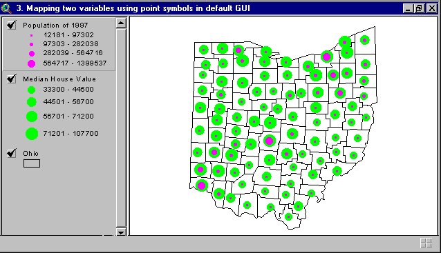
Figures 4 and 5 are examples of bivariate maps created by following the above procedure. Figure 4 uses graduated circles (a type of point symbols). The size of the circles on the top map ranges from 4 to 12 units. The size range of the bottom map is 14 to 20 units. Since the smallest circle on the bottom map is larger than the largest circle on the top map, the circular symbols of the top map will not completely block those of the bottom map. It makes the spatial distribution of both population and house value visible on the same display. Figure 5 uses two polygon symbols to map the same two variables. The symbol of the bottom map is graduated colors, while the top uses dot-filling patterns with varying densities. The densities of the dots are adjusted such that the graduated colors at the bottom are still visible.
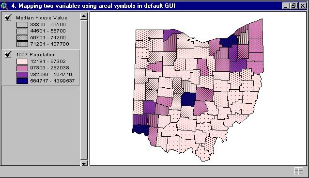
Both Figures 4 and 5 are not bivariate choropleth maps; they are only graphic overlays of two maps, each with a separate legend. A bivariate choropleth map has only one combined legend. The next section describes how the legend designed for one variable in ArcView can be modified to display two variables.
The mapping functions in ArcView are provided in a legend editor. Each map has an editable legend. The legend editor allows the user to classify a variable and assign graphic symbols to individual classes. The structure of the legend can be viewed as the following struct:
When a variable is classified into four classes, the value of Class is 1, 2, 3, and 4. Each value is associated with a graphic symbol and a label that includes the low limit and up limit of the class interval. The value of Class is not displayed in the legend (Figures 1 and 2). Another way to view the structure of legend is to convert the struct to a tabular format (Table 1).
Table 1. Structure of ArcView legend
|
Class |
Symbol |
Low Limit |
Up Limit |
|
1 |
Symbol 1 |
Low Limit 1 |
Up Limit 1 |
|
2 |
Symbol 2 |
Low Limit 2 |
Up Limit 2 |
|
3 |
Symbol 3 |
Low Limit 3 |
Up Limit 3 |
|
4 |
Symbol 4 |
Low Limit 4 |
Up Limit 4 |
This structure fits well to a single variable legend. To map two variables, it must be modified into the following (Table 2).
Table 2. Modified legend structure for bivariate choropleth mapping
|
Class |
Symbol |
Low Limit Var I |
Up Limit Var I |
Low Limit Var II |
Up Limit Var II |
|
1: I-1&II-1 |
Symbol I-1&II-1 |
Low Limit I-1 |
Up Limit I-1 |
Low Limit II-1 |
Up Limit II-1 |
|
2: I-1&II-2 |
Symbol I-1&II-2 |
Low Limit I-1 |
Up Limit I-1 |
Low Limit II-2 |
Up Limit II-2 |
|
3: I-1&II-3 |
Symbol I-1&II-3 |
Low Limit I-1 |
Up Limit I-1 |
Low Limit II-3 |
Up Limit II-3 |
|
4: I-1&II-4 |
Symbol I-1&II-4 |
Low Limit I-1 |
Up Limit I-1 |
Low Limit II-4 |
Up Limit II-4 |
|
5: I-2&II-1 |
Symbol I-2&II-1 |
Low Limit I-2 |
Up Limit I-2 |
Low Limit II-1 |
Up Limit II-1 |
|
6: I-2&II-2 |
Symbol I-2&II-2 |
Low Limit I-2 |
Up Limit I-2 |
Low Limit II-2 |
Up Limit II-2 |
|
7: I-2&II-3 |
Symbol I-2&II-3 |
Low Limit I-2 |
Up Limit I-2 |
Low Limit II-3 |
Up Limit II-3 |
|
8: I-2&II-4 |
Symbol I-2&II-4 |
Low Limit I-2 |
Up Limit I-2 |
Low Limit II-4 |
Up Limit II-4 |
|
9: I-3&II-1 |
Symbol I-3&II-1 |
Low Limit I-3 |
Up Limit I-3 |
Low Limit II-1 |
Up Limit II-1 |
|
10: I-3&II-2 |
Symbol I-3&II-2 |
Low Limit I-3 |
Up Limit I-3 |
Low Limit II-2 |
Up Limit II-2 |
|
11: I-3&II-3 |
Symbol I-3&II-3 |
Low Limit I-3 |
Up Limit I-3 |
Low Limit II-3 |
Up Limit II-3 |
|
12: I-3&II-4 |
Symbol I-3&II-4 |
Low Limit I-3 |
Up Limit I-3 |
Low Limit II-4 |
Up Limit II-4 |
|
13: I-4&II-1 |
Symbol I-4&II-1 |
Low Limit I-4 |
Up Limit I-4 |
Low Limit II-1 |
Up Limit II-1 |
|
14: I-4&II-2 |
Symbol I-4&II-2 |
Low Limit I-4 |
Up Limit I-4 |
Low Limit II-2 |
Up Limit II-2 |
|
15: I-4&II-3 |
Symbol I-4&II-3 |
Low Limit I-4 |
Up Limit I-4 |
Low Limit II-3 |
Up Limit II-3 |
|
16: I-4&II-4 |
Symbol I-4&II-4 |
Low Limit I-4 |
Up Limit I-4 |
Low Limit II-4 |
Up Limit II-4 |
Table 2 shows a general structure for a bivariate choropleth map in which each variable is classified into four classes. Not all the possible sixteen classes may necessarily appear on the map, especially when the two variables correlate. With this modified legend structure, the remaining question is how to apply it to create bivariate choropleth maps. The next section describes an algorithm for creating bivariate choropleth maps and the implementation of the algorithm in Avenue.
The following algorithm is developed for bivariate choropleth mapping.
Low Limit–Up limit (Variable I)&Low Limit–Up Limit (Variable II)
This algorithm is implemented in an Avenue script, which is then converted into an ArcView extension named Bivariate.avx. The extension will be downloadable from Esri’s web site. Figure 6 is a bivariate choropleth map created with this extension.
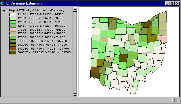
The Bivariate extension is the first Avenue script/extension for creating bivariate choropleth maps. With this extension, it is anticipated that choropleth bivariate mapping, as a powerful cartographic technique, will be widely used in the GIS community.