Site selection of petroleum pipelines has historically focused on lessening the cost of construction and increasing the efficiency of transport. This paper demonstrates how GIS can be used in the site location process to minimize impacts to the environment during construction and from accidental release, as well as to lessen the costs of permits and liability risks associated with accidental releases. Ecological variables developed from publicly available spatial data sets are utilized in this process.
Introduction
The oil and gas industry is increasingly using GIS technology in siting new pipelines as a tool to lessen both construction and operational costs (Hicken et al., 1998). The themes and variables used as input in this process mainly address direct construction costs and pipeline efficiency once the pipeline has been completed. Some of the variables examined include:
What is usually not taken into account in the siting process is the potential costs of environmental impacts during construction as well as ecological and liability costs that may result from accidental releases after construction has been completed. Some of these costs can be substantial (potentially millions of dollars) and include:
Over the past few years, an increasing number of environmental spatial data sets have become available to the general public, offering a great opportunity for companies to avoid these environmental and liability risks with relatively little effort by incorporating them into their normal GIS siting procedures. This paper provides guidance on the environmental spatial data sets available to the public (many over the internet) and examines some of the attributes that may be used in the siting process to lessen impacts to the environment, minimize the risk of damage to the pipeline (e.g., from erosion, debris, or third party damage), and reduce liability in the event of an accidental release. In addition, this process may also help to lessen permitting costs and identify sections of existing pipeline where additional preventive measures may be needed. First, we examine some of the environmental criteria, spatial data sets, and attributes that should be considered and where this data can be obtained, then conclude with an example utilizing many of the data sets outlined. It is important to mention that the criteria used in this paper are meant to augment rather than replace the traditional site selection criteria. Furthermore, the list provided is to be used as a guide and is not meant to be all-inclusive.
In addressing environmental concerns, there are three main objectives:
Ecological Parameters and Data Sets
Pipeline Vulnerability
Pipelines are vulnerable to damage when exposed. Pipeline cover may be lost where a pipeline is near water features such as tidal areas or river crossings. Loss of cover may result because of erosion from river meandering, undercutting, or flooding. Additionally, during peak flows, suspended sediment, soil, and debris such as logs and limbs can cause damage through abrasion. Pipeline damage may also result from external forces applied to a pipeline from third party activities (e.g., heavy machinery use). Information sources available for assessing pipeline vulnerability risks are listed below.
Flood information. Classifies high-risk areas as Flood Hazard Areas. This data can be purchased from the Federal Emergency Management Agency (FEMA) (appendix A). Data for much of the United States is available in hard copy maps, and approximately 30% are available in digital form (Q3 data) at a scale of 1:24,000.
Peak stream flows. This information can be used not only to differentiate between the size of streams, but also to help avoid construction during high flows, thereby reducing impact to the environment and construction costs. Base discharge and peak discharge information is available for free over the internet from the U.S. Geologic Survey for stream gaging stations throughout the United States (appendix A).
Areas of urban density. Areas with high urban density may increase the liability risk in the event of an accidental release. Data sets such as Metropolitan Statistical Areas and Census Block Tracts/Groups can be used for determining proximity to high-density population areas. Spatial data sets (TIGER files) are available from the U.S. Census Bureau and include Metropolitan Areas, Urbanized Areas, Census Tracts, and Census Block Groups. These data sets can be downloaded or ordered over the internet at varying costs and scales ranging from 1:100,000 and smaller (e.g., 1:5,000,000 which is free) (appendix A). Some of this data (Census tracts, census block groups, etc.) is also provided on CD-ROM from Esri and included with the purchase of ArcView (Esri Data & Maps) at varying levels of detail (Esri, 1998).
Land zoning. Areas zoned for commercial or residential development may be useful for determining risks from third party damage from future construction activities. Zoning data is available from state, county, or local governments. As many of these agencies are beginning to utilize GIS technology, this data is increasingly available in digital form.
Land use/land cover. Land use/land cover themes provide information on general cover and land use that may be used in lieu of or to supplement zoning and urbanized areas. This theme can be used to help identify those areas of higher risk of third party damage as well as areas that have a relatively low risk. In addition, this theme can help identify areas to minimize construction costs. Land use/land cover classifications include urban or built-up land, residential, commercial services, industrial, transportation/communications, industrial and commercial, mixed urban or built-up land, other urban or built-up land, agricultural land, cropland and pasture, orchards/groves/vineyards/nurseries, confined feeding operations, other agricultural land, rangeland, herbaceous rangeland, shrub and brush rangeland, mixed rangeland, forest land, deciduous forest land, evergreen forest land, mixed forest land, water, streams and canals, lakes, reservoirs, bays and estuaries, wetland, forested wetlands, nonforested wetlands, barren land, dry salt flats, beaches, sandy areas other than beaches, bare exposed rock, strip mines/quarries/gravel pits, transitional areas, mixed barren land, tundra, shrub and brush tundra, herbaceous tundra, bare ground, wet tundra, mixed tundra, perennial snow and ice, perennial snowfields, and glaciers (USGS, 1990). Land use/land cover data is available for free over the internet from the USGS GeoData site and the Environmental Protection Agency (EPA) (appendix A). These are generally at a scale of 1:250,000, although a limited number of areas are available at 1:100,000. While the small-scale data may be too general for final site selection, it may be useful as an initial filter in the siting process. However, larger scale data (up to 1:24,000) is becoming available for free or purchase from individual state agencies such as Departments of Natural Resources.
Slope. Slope data can be used to determine areas of high erosion potential. Digital elevation model (DEM) data used to calculate slope is available for free over the internet from USGS at varying scales (1:24,000 in many areas) (appendix A).
Soils. Soils data at varying scales (from 1:24,000 and smaller, e.g., STATSGO and SSURGO) is available from state and county agencies (e.g., Departments of Natural Resources) as well from the U.S. Department of Agriculture Natural Resource Conservation Service (USDA-NRCS) over the internet (appendix A) for many regions in the United States. Soils information may help identify regions where corrosion risk is high and, in conjunction with slope, may help determine risk of erosion.
Ecologically Important Areas
Wetlands. Wetlands are ecologically important areas with national significance (societally important) because of the historical losses from development, and the ecological services they provide including habitat for migratory waterfowl and amphibians. Wetlands provide water for storage, aquifer recharge, water cleansing, aquatic and nonaquatic species reproduction, cover, and feeding. Additionally, they are sensitive to petroleum discharges because of limited dilution (small size, limited water exchange). The National Wetlands Inventory (NWI) maintains a spatial database of wetland areas with alphanumeric codes identifying the type of wetland feature (appendix A). The NWI has mapped 89% of the area of the lower 48 states. About 39% of the area of the lower 48 states are available in for free over the internet in digital form at a scale of 1:24,000.
Areas of special status species. Areas that support rare species and rare and/or relatively natural plant and animal communities provide reservoirs of genetic diversity and ecological integrity, and thus require special protection. National Heritage Programs provide lists of locations of (1) federally listed threatened or endangered species, (2) state or local species of special concern, and (3) areas containing habitats or natural communities of ecological significance. Additional sources of information include the US Fish and Wildlife Service Division of Endangered Species (appendix A) and the U.S. National Park and Forest Services.
Water features. Flowing water, ponds, lakes, and reservoirs provide ecological services and nonuse values, including (1) recreation (hunting, fishing, swimming, boating); (2) aquatic and nonaquatic species reproduction, cover, and feeding; and (3) water and sediment quality. Water features can serve as a conduit for spilled oil, as well as being ecologically important. Water features are available for free from the USGS internet site (appendix A) in the form of digital line graphs (DLGs). The attributes relevant to water features include (major and minor codes) area to be submerged (050 0108); marsh, wetland, swamp, or bog (050 0200); mangrove area (050 0112); bay (050 0112); gut (050 0122); shoreline (050 0207); manmade shoreline (050 0201); indefinite shoreline (050 0203); apparent shoreline (050 0421); stream (050 0412); ditch or canal (050 0414); channel (050 0419); lake or pond (050 0421); right & left bank (050 0605-6); intermittent (050 0610); submerged (050 0612) (USGS, 1999b).
Public Lands and Recreation Areas
Many public lands and recreation areas provide important ecological and societal services and values and should therefore be considered in the siting process. Publicly owned lands include national, state, city, or county forests, grasslands, seashores, monuments, parks, refuges, recreation areas, and wilderness areas. Information on public lands is provided in the digital line graph (DLG) boundary files and is available for free from the USGS internet site (appendix A).
Other Features and Data Sources
In addition to the features and data sources listed above, there are several other sources of data that can be helpful in the siting and mitigation process.
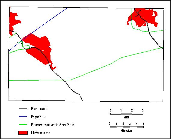
Roads, trails, railroads, and utilities. The location of roads, trails, and railroads can play a significant role in reducing costs and limiting environmental impacts during pipeline construction. Siting a pipeline near existing road networks will minimize the creation of new roads during construction and for maintenance. Attribute information attached to the linework (such as width of roads) can be used to minimize construction costs and impacts to the environment. In addition, utilizing existing utility corridors instead of creating new ones, can reduce both construction costs and environmental impacts can be reduced (although the rights to the easements would need to be taken into consideration). These themes are publicly available for free from the USGS as DLG files at scales from 1:24,000 and smaller (appendix A).
Satellite and aerial photos. Remotely sensed data from satellites (e.g., Landsat and SPOT) and aerial photography is widely available from public and private sources (appendix A) at varying scales. As many of the data sets listed above are available for only portions of the country, remotely sensed data can be used as a source for many of these themes (e.g., hydrology, wetlands, land use/land cover, urban areas, etc.) or to enhance data that was unavailable at the scale needed. The thematic data sets needed can be extracted from the imagery by either on-screen digitizing or automated and semi-automated classification methods. Vegetative cover may also be derived and may help guide the site location away from heavily forested areas.
Digital orthophotos and digital raster graphics. In contrast to the remotely sensed data listed above that may require extensive processing and expertise to use, the USGS provides orthorectified aerial photos (DOQ) and rectified scanned topographic maps (DRG), either for free (DRG) or for a nominal cost (DOQ) (appendix A) over much of the country. While it may or may not be possible to extract the thematic information needed in an automated fashion from these data sets, many of the themes listed above can be obtained by on-screen digitizing or by visual evaluation. These sources of data can also be used to evaluate the accuracy of the thematic layers. In addition, these data sets can provide information that is unavailable in other data sets (e.g., locations of isolated buildings, etc.). The spatial resolution of these data sets is often much greater than can be obtained from satellite imagery (up to 1 meter for DOQ and 1:24,000 for DRG).
Hard copy sources. Many of the data sets listed above that are not available for a specific region of the county may be available in hard copy form. By scanning or digitizing these maps, they can be incorporated into the GIS procedure. However, even if they aren�t utilized in a digital format, the data can be used to visually guide the siting process.
Case Study
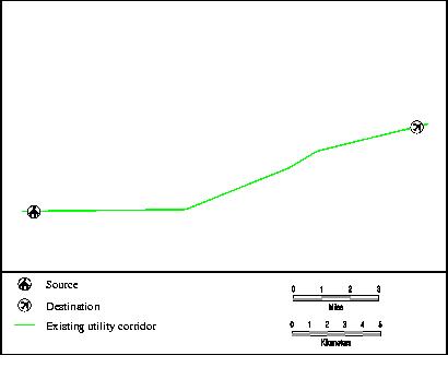
The case study outlined below is intended to illustrate the process of acquiring, processing, and implementing a pipeline siting procedure in a GIS. The basic problem addressed is this case study is as follows. Assuming that an existing utility corridor might realistically be used to site a pipeline between source and destination points (given land easement costs, etc.) (Figure 1), where could a pipeline be sited between these same two points that would result in the least environmental impact and liability risks given spatial data that is available for free over the internet? Since the purpose of this paper is to show how GIS can be used to minimize environmental impacts and liability risks, this case study utilized mainly environmental data sets and attributes and a minimal attempt was made to address engineering parameters related to construction or operating efficiency.
Figure 1. Existing utility corridor theme converted from USGS DLG files (USGS, 1999b).
Data Acquisition
The first step in the process is to acquire all the data sets needed at the scale desired. Many of the data sets available are indexed by county or USGS quadrangle index and therefore, digital topographic indexes at 1:250k, 1:100k, and 1:24k should be used in conjunction with digital state and county data to facilitate the download process.
Two adjacent USGS 1:24,000 topographic quadrangles were selected from the southeastern United States. The criterion used to select these was based solely on the availability of as many themes as possible at the largest possible scale. All data sets used in the analysis were available for free over the internet. Table 1 describes the sources and data sets acquired.
Table1. Data sets acquired
|
Description |
Source |
Format |
Scale |
|
Transportation |
USGS GeoData Internet Site |
DLG-SDTS |
1:24,000 |
|
Railroads |
USGS GeoData Internet Site |
DLG-SDTS |
1:24,000 |
|
Utility and Pipelines* |
USGS GeoData Internet Site |
DLG-SDTS |
1:24,000 |
|
Public Land Boundaries |
USGS GeoData Internet Site |
DLG-SDTS |
1:24,000 |
|
Digital Elevation Model (DEM) |
USGS GeoData Internet Site |
SDTS-Raster Profile |
30 meter |
|
National Wetlands Inventory (NWI) |
Fish & Wildlife Service, National Wetlands Inventory Internet Site |
ARC/INFO Export |
1:24,000 |
*Data used for comparative purposes only.
Data Processing
After the data were downloaded for each quadrangle from the sites, each theme was imported into either ARC/INFO coverage format (vector themes) or grid (DEMs), and all associated attribute files were joined with the appropriate feature attribute tables. In addition, because many of the data sets contained cryptic alphanumeric attribute codes (DLG and NWI), lookup tables were created from metadata sources.
After the data had been converted into coverages, the individual quadrangles were joined together (using "mapjoin" or "append" for vectors, and "mosaic" for grids) to create seamless coverages for each theme. The appended themes were then checked for errors and any artificial polygon boundaries created from the merge were removed by running "dissolve." All coverages and grids were also projected into a common projection system. The processed themes used in the analysis are shown in Figures 2a-d.
Figure 2a. USFWS National Wetlands Inventory (NWI) theme (USFWS, 1999a).
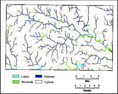
Figure 2b. Digital elevation model (DEM) data converted from USGS SDTS files (USGS, 1999a).
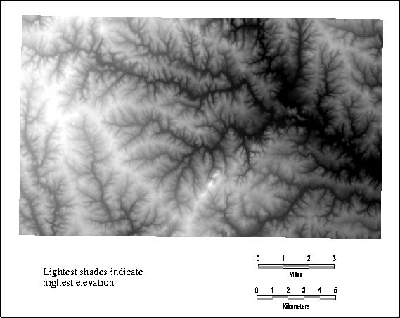
Figure 2c. Transportation theme converted from USGS DLG files (USGS, 1999b).
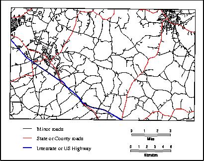
Figure 2d. Railroad, public land boundary, and utility/pipeline themes converted from USGS DLG files (USGS, 1999b).
Because the linework between the DLG hydrology and the NWI data was essentially the same, and a higher degree of discrimination could be obtained from the NWI attributes, the DLG hydrology was used for verification purposes only.
Classification and Costing
All unique codes were identified for each theme by running a frequency on the appropriate attribute field. NWI arc and polygon theme were separated and processed individually. Slopes derived from the DEM were grouped into three classes: 0-10%, 10-20%, and 20-30% (there were no slopes greater than 30% in this data set). Each polygon, line, and slope class was then subjectively assigned a relative cost on a scale of 0 to 5 based on their vulnerability (least to most) to environmental degradation in the event of an accidental release or during the construction process. The criterion used in assigning costs was based on (1) potential loss of recreation value, (2) potential loss of ecological function, (3) potential of feature to transport released petroleum, and (4) relative effort required to remediate. The costs of stream and transportation crossings were also incorporated into this structure. In addition to the cost attribute, sensitive ecological areas such as wetlands, streams, and lakes were buffered by 150 meters (492 feet) to limit the risk of environmental damage. The cost and buffer assignments are summarized in Table 2.
Table 2. Classification (USFWS, 1999b and USGS, 1990a) and relative cost assignments.
|
Theme |
Attribute (code) |
Description |
Costa |
Buffera (m) |
|
NWI |
Lacustrine, limnetic, and littoral (L1/L2) |
Wetlands and deepwater habitats with all of the following characteristics: (1) situated in a topographic depression or a dammed river channel; (2) lacking trees, shrubs, persistent emergents, emergent mosses, or lichens with greater than 30% area coverage; and (3) total area exceeds 20 acres. |
5 |
150b |
|
NWI |
Palustrine, aquatic bed (PAB) |
Nontidal wetlands with plants growing on or below surface. Water less than 2 meters deep. |
5 |
150 |
|
NWI |
Palustrine, emergent (PEM) |
Nontidal wetlands with erect, rooted, herbaceous hydrophytes, excluding mosses and lichens. |
5 |
150 |
|
NWI |
Palustrine, forested (PFO) |
Nontidal forested wetlands. |
3 |
150 |
|
NWI |
Palustrine, scrub shrub (PSS) |
Nontidal wetlands with scrub shrub vegetation. |
4 |
150 |
|
NWI |
Palustrine unconsolidated bottom (PUB) |
Nontidal wetlands with at least 25% cover of particles smaller than stones and vegetation cover less than 30%. |
3 |
150 |
|
NWI |
Palustrine unconsolidated shore (PUS) |
Nontidal wetlands including landforms such as beaches, bars, and flats. |
3 |
0 |
|
NWI |
Riverine lower perennial (R2) |
Riverine system characterized by low gradient and slow water velocity. Substrate mainly sand and mud. Well developed floodplain. |
3 |
150 |
|
NWI |
Riverine upper perennial (R3) |
Riverine system characterized by high gradient and fast water velocity. Very little floodplain development. |
5 |
150 |
|
NWI |
Riverine intermittent (R4) |
Intermittent riverine system including channels that contain flowing water only part of the year but may contain isolated pools when the flow stops. |
2 |
0 |
|
NWI |
Uplands (U) |
Uplands. |
0 |
0 |
|
Transportation |
Primary route (1700202) |
Interstate or U.S. highway. |
5 |
0 |
|
Transportation |
Secondary route (1700205) |
State or county highway. |
4 |
0 |
|
Transportation |
Road class 3 (1700209) |
Class 3 road or street. |
2 |
0 |
Table 2. Classification (USFWS, 1999b and USGS, 1990a) and relative cost assignments, continued.
|
Theme |
Attribute (code) |
Description |
Costa |
Buffera (m) |
|
Transportation |
Road class 4 (1700210) |
Class 4 road or street. |
2 |
0 |
|
Transportation |
Cloverleaf or interchange (1700402) |
Cloverleaf or interchange. |
5 |
0 |
|
Transportation |
Nonstandard road (1700405) |
Nonstandard section of road. |
1 |
0 |
|
Transportation |
Cul-de-sac (1700005) |
Cul-de-sac. |
5 |
0 |
|
Railroad |
Railroad (1800201) |
Railroad. |
3 |
0 |
|
Railroad |
Railroad siding (1800208) |
Railroad side track. |
3 |
0 |
|
Urban |
Incorporated city, town (0900101) |
Urban. |
5 |
0 |
|
Slope |
Class 1 |
Slope 0-10%. |
0 |
0 |
|
Slope |
Class 2 |
Slope 10-20%. |
2 |
0 |
|
Slope |
Class 3 |
Slope 20-30%. |
4 |
0 |
a
All costs and buffers are relative and values are for illustrative purposes only.b
For simplicity, all buffers used were 150 meters.As mentioned above, the buffers and costs assigned to each feature were subjectively assigned. The following examples illustrate the rationale used to assign a cost and buffer to several of the features used in the analysis. Lake and nontidal wetlands with aquatic bed and emergent features (NWI codes L1/L2, PAB, PEM) were assigned the highest relative cost (5) and buffer (150 meters) because of their high ecological function and importance as habitat as well as their recreational value (fishing, boating, scenery, etc.). In addition, a spill in this environment would be costly because all the lakes in the study area are relatively small and therefore would have little dilution. Similarly, wetlands with emergent/aquatic vegetation were assigned the highest cost and buffers because of their high ecological value as habitat for waterfowl and amphibians, their ability to cleanse water, and as habitat for aquatic and nonaquatic species reproduction. These environments also provide recreation activity in the form of hunting. In contrast, forested wetlands (PFO) were assigned a lower cost. While still a wetland, this type of environment was perceived as less ecologically important than the emergent wetland (less vegetation) and offered less recreation value. The highest cost and buffer was also assigned to fast-flowing river environments (R3). While these features provide less ecological function than the lake or wetland environments, their ability to transport large quantities of released petroleum and therefore their potential to damage many miles of stream habitat require assignment of the highest degree of protection. A similar rationale was used in assigning costs to the other environmental features. Finally, the costs assigned for transportation and railroad features were based solely on a relative estimate of construction costs. Therefore, the larger the road, the higher the cost.
Determination of Least-Cost Path
Relative cost and buffer values assigned to the attribute tables of the vector coverages were then converted into raster format, with each buffer assigned the appropriate cost value. For the NWI coverages, this was achieved using the "eucallocation" function in grid, which was run separately for the line and polygon features. Rasterization of the transportation and railroad layers was achieved by simply assigning the "cost" value to the output grid during the conversion process. A cell size of 5 meters was used for all raster themes so that linear features would not be over-represented (including the slope grid that was resampled).
The cost grids for each theme were then combined into a single layer, with each output cell location receiving the summation of all other grid cells for that location. For example, for a given cell location, if the transportation layer with a cost value of 5 (interstate highway) intersected a slope with a cost value of 4 (20-30%), the resultant output cell value would be 9. Individual and summary cost grids are shown in Figures 2a-e.
Figure 3a. Polygonal NWI features, gridded by relative cost value.
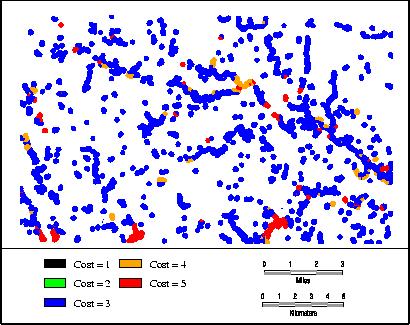
Figure 3b. Linear NWI features, gridded by relative cost value.
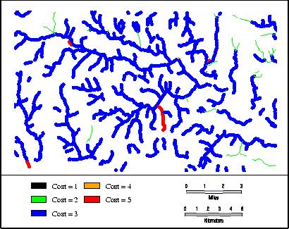
Figure 3c. Transportation routes, railroads, and urban areas gridded by relative cost value.
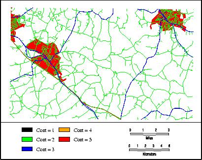
Figure 3d. Slope classes, gridded by relative cost value.
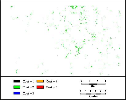
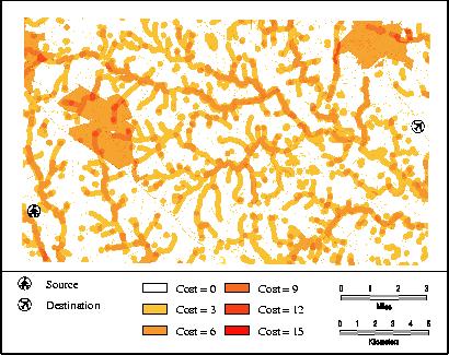
Figure 3e. Final relative cost grid, containing the summation of individual cost themes.
Additional grids were created to provide the source and destination locations for the pipeline route. As mentioned above, these locations were chosen at the endpoints along an existing utility corridor so that the two routes could be compared. The source grid and the summation grid of costs were used as inputs into the GRID function "costdistance." The output of this function is a cost accumulation grid in which each cell value is the accumulated cost to the closest source cell. This output was then used as input into the "costpath" function to derive a least-cost path grid. The syntax used for these functions is shown as:
Grid: pipeaccum = costdistance(pipesrcg, pipecost, pipeback, pipealloc, #, pipesrcg)
where "pipecost" is the summed cost grid, and "pipesrcg" is the source grid.
Grid: pipepath = costpath(pipefromg,pipeaccum,pipeback,bylayer)
where "pipefromg" is the destination grid, "pipeaccum" is the output from the costdistance function, "pipeback" is a grid that can be used to reconstruct a route to the source, and "bylayer" is an option that specifies the single least-cost path as output.
Results
The final least-cost route overlaid on the total cost grid is shown in Figure 4. The black line represents the path that would provide the best protection against environmental impact during construction or from an accidental release given the weighting parameters used, and the green line represents an existing utility corridor that might be used to site a pipeline using traditional methods.
Figure 4. Utility corridor route and relative least-cost route overlaid on total relative cost grid.
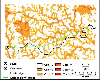
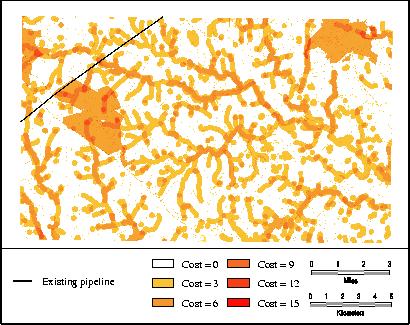
Since the path shown represents only environmental parameters, it does not necessarily show the optimal site location given engineering, land easement, and other costs (e.g., efficiency of transport) that would be used in the normal siting process. However, while use of the entire path shown is probably not desirable, the use of individual portions would provide some ecological benefit. In addition, by overlaying existing pipelines on the total cost layer (Figure 5), areas where the pipeline crosses ecologically sensitive areas can be identified as potential locations where additional monitoring or mitigation measures might be beneficial.
Figure 5. Existing pipeline overlaid on the total cost grid.
Further Refinement
In comparing the two routes, an obvious refinement to the model would be to incorporate a parameter that takes into account the total length of the pipeline. Such a modification would probably create a more realistic path. In addition, a much more extensive cost structure based on scientific and engineering parameters that better approach reality would need to be developed. Ultimately, by incorporating both the environmental and traditional sets of criteria into a costing structure similar to the one above, an optimal route could be achieved. Finally, it should be mentioned that in the traditional siting process where GIS is used, many of the data sets used in this case study have already been acquired. The addition of a few more layers related specifically to the environment would therefore require minimal additional effort, and the potential savings could be enormous.
Appendix A. Sources and locations of data sets.
|
Data |
Source |
Internet Location |
|
Census data (TIGER) |
U.S. Census Bureau |
http://www.census.gov/geo/www/tiger/ or http://www.census.gov/geo/www/cob/ |
|
Endangered species data |
U.S. Fish and Wildlife Service Division of Endangered Species |
http://www.fws.gov/r9endspp/endspp.html |
|
Flood information (Q3 data) |
Federal Emergency Management Agency (FEMA) |
http://www.fema.gov/msc/ordrinfo.htm |
|
Hydrology, transportation, land use/land cover, public ownership, digital elevation model (DEM) |
U.S. Geological Survey (USGS) |
http://edcwww.cr.usgs.gov/doc/edchome/ndcdb/ndcdb.html |
|
Land use/land cover |
U.S. Environmental Protection Agency (EPA) |
ftp://ftp.epa.gov/pub/spdata/EPAGIRAS/ |
|
National Wetlands Inventory (NWI) |
U.S. Fish and Wildlife Service |
http://www.nwi.fws.gov |
|
Orthorectified aerial photography |
Digital Orthophoto Quad (DOQ) |
http://edcwww.cr.usgs.gov/webglis |
|
Satellite imagery |
Landsat satellite data |
http://geo.arc.nasa.gov/sge/landsat/landsat.html or http://edcwww.cr.usgs.gov/webglis |
|
Satellite imagery |
SPOT Image |
http://www.spot.com/spot/spot-us.htm |
|
Scanned topographic maps |
Digital Raster Graphics (DRG) |
http://mcmcweb.er.usgs.gov/drg/avail.html#online |
|
Soils data |
USDA-NRCS |
http://www.ftw.nrcs.usda.gov/soils_data.html |
|
Stream flow data (stream gaging data) |
U.S. Geological Survey (USGS) |
http://water.usgs.gov |
References
Environmental Systems Research Institute. 1998. Esri Data and Maps. Environmental Systems Research Institute. Redlands, CA.
Hicken, J.E., T. Krumbach, N. Dahman, and J. Gage. 1998. Use of High Resolution Remote Sensing for Gas Line Route Selection, Visiting Investigator Program Affiliated Research Center (VIP/ARC) Final Report. Prepared for Wisconsin Power and Light (WP&L) and Environmental Remote Sensing Center (ERSC). Board of Regents of the University of Wisconsin System, University of Wisconsin-Madison.
USFWS. 1999a. National Wetlands Inventory Inventory 1:24,000 digital data. [ftp://www.nwi.fws.gov/arcdata.]
USFWS. 1999b. National Wetlands Inventory, Wetcodes.exe. [ftp://www.nwi.fws.gov/maps]
USGS. 1990a. Digital Line Graphs From 1:24,000-Scale Maps, Data Users Guide 1, Appendix D, DLG attribute codes.
USGS. 1990b. Land Use And Land Cover Digital Data From 1:250,000- and 1:100,000-Scale Maps, Data Users Guide 4, U.S. Geological Survey Land Use and Land Cover Classification System for Use with Remote Sensor Data.
USGS. 1999a. 1:24,000 Digital Elevation Model data. [http://edcwww.cr.usgs.gov/doc/edchome/ndcdb/ndcdb.html]
USGS. 1999b. 1:24,000 Digital Line Graph data. [http://edcwww.cr.usgs.gov/doc/edchome/ndcdb/ndcdb.html]