
James A. Kuiper and Konnie L. Wescott
A GIS Approach for Predicting Prehistoric Site Locations *
Presented at the Nineteenth Annual Esri User Conference,
San Diego, California, USA
July 26-30, 1999
Sponsored by Environmental Systems Research Institute
(Esri)
| The submitted manuscript has been created by the University of Chicago as Operator of Argonne National Laboratory ("Argonne") under Contract No. W-31-109-ENG-38 with the U.S. Department of Energy. The U.S. Government retains for itself, and others acting on its behalf, a paid-up, nonexclusive, irrevocable worldwide license in said article to reproduce, prepare derivative works, distribute copies to the public, and perform publicly and display publicly, by or on behalf of the Government. |
* Work supported under a military interdepartmental purchase request from the U.S. Department of Defense, through U.S. Department of Energy contract W-31-109-Eng-38.
ABSTRACT
Use of geographic information system (GIS)-based predictive mapping to locate areas of high potential for prehistoric archaeological sites is becoming increasingly popular among archeologists. Knowledge of the environmental variables influencing activities of original inhabitants is used to produce GIS layers representing the spatial distribution of those variables. The GIS layers are then analyzed to identify locations where combinations of environmental variables match patterns observed at known prehistoric sites. Presented are the results of a study to locate high-potential areas for prehistoric sites in a largely unsurveyed area of 39,000 acres in the Upper Chesapeake Bay region, including details of the analysis process. The project used environmental data from over 500 known sites in other parts of the region and the results corresponded well with known sites in the study area.
INTRODUCTION
Use of geographic information systems (GISs) for predictive mapping to locate unrecorded prehistoric archaeological sites is becoming increasingly popular among archeologists. Generally, these techniques assume that the selection of sites by original inhabitants was at least partially based on a set of favorable environmental factors, such as distance to water or topographic setting. Another assumption is that modern day GIS layers consistently characterize changes from the prehistoric condition of the region sufficiently well that they can be used to help discover additional sites.
Predictive modeling uses deductive and inductive approaches. Deductive models are based on theories about the behavior of the prehistoric inhabitants. Inductive models, which are more commonly used, are based on observed patterns in ground surveys or other data. One of the more powerful and widely used inductive techniques is logistic regression. This rigorous statistical approach requires an adequate sample size, and independent variables must be measured both for areas known to have sites and areas known to lack sites (non-site data). Some archaeological surveys are now being designed specifically to support logistic regression in GISs by more systematically collecting environmental information and by including records of surveyed areas where sites were not found (BRW 1996).
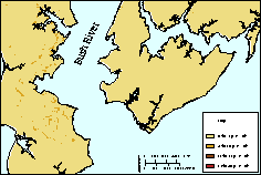
In situations where available data must be used, the requirements for logistic regression may not be met, but inductive predictive modeling is still possible with alternative methods and can achieve useful results. This paper illustrates such a situation. The case study described here was conducted for Aberdeen Proving Ground (APG), a U.S. Army test site in the Upper Chesapeake Bay area (Figure 1). Established in 1917, APG is used for testing artillery and other ordnance, military vehicles, and a wide variety of other equipment. The land area is about 39,000 acres, of which over 25,000 acres consists of wetlands or woodlands where natural and cultural resources are present and protected. In contrast, much of the adjacent land area outside APG has continued to be intensively farmed and recently has become increasingly urbanized. Despite the relatively protected setting and the reduced amount of disturbance on APG, archaeological surveys have been limited because of mission activities.
The 46 known prehistoric archaeological sites at APG are predominantly shell middens and lithic scatters, although some sites also contain ceramics. The sites range in age from Paleo-Indian to the Late Woodland/Contact period. These sites occur predominantly along the coast, with over 90% within 50 meters of a shoreline or stream. Bias in the population of known APG sites exists because most surveys were made along shorelines. Inland areas are almost completely unsurveyed.
In the upper bay region outside of APG, many sites have been found in areas with similar environmental characteristics to APG. Known characteristics of these sites provided a basis for designing a predictive model for APG to determine site potential in unsurveyed areas.
Despite the unique character of the APG site, a wealth of environmental GIS information (Kuiper 1996; DSHE 1996), over 500 known sites in the region, and the likelihood of many undiscovered prehistoric archaeological sites on APG, the preconditions for logistic modeling could not be met. The study was limited to available data, and logistic regression could not be used because of the lack of non-site environmental data, and because the sample size of known sites was not sufficient unless the model was reduced to a very simple set of environmental conditions. A general guideline for logistic regression is to average at least 25 samples for each unique environmental condition, with less than 20% having under 5 samples (SAS 1990). To conduct the modeling, an alternative approach was developed that took into account the environmental characteristics of the known sites and the spatial distribution of those characteristics, without using logistic regression to calculate the results.
THE MODELING APPROACH
Preparation for modeling began with collection of data and the process of distilling it into a useful form for modeling. This process included developing an archaeological site database, compiling GIS layers representing spatial distributions of environmental variables recorded for known sites, and examining the data with descriptive statistics. The statistical results were used to decide the environmental layers to use for model calculations and the model parameters. Finally, the model was run and results were visualized and compared to known sites on the APG installation.
Archaeological Site Database
Information for 572 recorded prehistoric sites in the Upper Chesapeake Bay region was first tabulated in a database and then processed with Statistical Analysis System (SAS) software for analysis (Wescott and Kuiper 1999; MHT 1995). The region that these sites were found in was assumed to have similar characteristics to APG at this stage, but analysis to verify this assumption was performed later in the study. Site data included a polygon location in the GIS, site type, distance to water, type of water source (brackish or fresh), soil type, topographic setting, slope, elevation, aspect, geomorphic setting, time period, dimensions, and contents. The data were examined with statistical software to better understand the information and to identify patterns that would be useful for modeling purposes. A separate analysis was made for shell midden sites and other sites (non-shell) to reduce the effect of competing variables where a positive factor for one type of site is a negative factor for another. Locations of sites and survey areas were also mapped in the GIS and linked to the site database.
Production of Environmental GIS Layers
GIS layers for each of the environmental variables in the archaeological site database were produced. Most layers were derived from existing line or polygon layers, but some required a number of steps to produce the final result.
Distance to Water
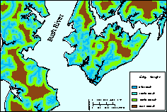
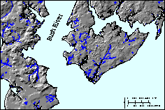
The distance-to-water layer was produced from a generalized hydrology layer in the GIS (Figure 2). Small channels and known man-made channels were removed and polygons indicating land vs. water were created. Arc LINEGRID was used to produce a raster version of the lines and Arc POLYGRID produced a similar version of the polygons. Grid EUCDISTANCE calculated distances from the shorelines, and then areas covered with water were reassigned a distance of 0 using the Grid CON function. Once the water source type layer was completed, a similar process was used to produce a distance to brackish water layer to improve the results of the shell midden model (Figure 3).
Type of Water Source
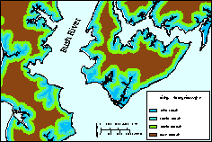
The type-of-water layer, in conjunction with distance to water, was expected to be useful in predicting sites, but required more analysis and processing to derive from available GIS information. Shorelines in the hydrology layer used for distance to water were manually coded into divisions for bay, river, creek, and lake/pond. (The Gunpowder and Bush Rivers widen in the APG area and are brackish.) Water chemistry data in the U.S. Fish and Wildlife Service National Wetlands Inventory (NWI) polygons were used to identify additional brackish water bodies. Arc BUFFER was used with a small distance to produce areas around the linear features. The layer then contained polygons with the following water source categories: bay shoreline, river shoreline, brackish/salt creek shoreline, and fresh creek shoreline. Arc POLYGRID was used to produce a raster version of the layer, and Grid EUCALLOCATION was used with a distance of 1,000 ft to identify the water source type of all land areas within 1,000 ft of a major water source. The remaining land area was then coded as having no major water source with the Grid CON function. Figure 4 depicts the type-of-water source layer for a portion of the APG site.
Soil Type
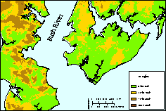
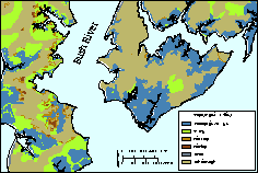
Soil survey data for most of APG dates to 1927, presumably because of many of the same access and safety issues that limit archaeological surveys. This soil survey is at a scale of 1:62,500 and has a low level of detail for APG. A small portion of the site is in Baltimore County, however, and 1976 survey data at a scale of 1:20,000 were available for that area. Production of this GIS layer required simply coding the soil categories with numeric values that could be used in a raster format and grouping soil types to match the more general categories in the archaeological site data. The result is shown in Figure 5.
Elevation, Slope, and Aspect
A digital elevation model (DEM) for the full site existed in the GIS database (Figure 6). It was produced from elevation lines and points using Arc TOPOGRID for the purpose of watershed modeling. Source data for the DEM were 2-ft contour lines and point elevations for the Aberdeen peninsula and 5-ft contour lines for the Edgewood peninsula and the other APG areas. Grid RESAMPLE was used with the 'cubic' option to convert the DEM from 25-ft cells to 100-ft cells for the model. The slope layer (Figure 7) was calculated directly from the DEM by using Grid SLOPE with the 'percentrise' option. Aspect (Figure 8) was produced with the Grid ASPECT command, and the output azimuth values were reclassified into eight values for the cardinal directions used in the archaeological site data.
Topographic Setting
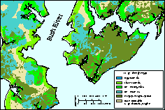
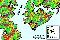
The topographic setting was an important element of the environmental information in the archaeological site database, but it was challenging to produce a GIS layer with the appropriate categories identified. Topographic settings found in the archaeological site database were examined and placed into the following more general categories: beach, floodplain, inland flat, bluff, hilltop, terrace, and hill slope. Beach areas were defined by applying a 25-ft buffer to NWI "unconsolidated shore" polygon and line features. Floodplains were produced by extracting areas with slopes less than or equal to 5 percent from the DEM and eliminating areas not adjacent to a shoreline. Bluffs, hill tops, and terraces were added to the map manually using several layers for guidance. These layers included contours, slope, shaded relief derived from the DEM, and hydrology (Figure 9). Hill slopes were derived from the DEM by using slopes over 5 percent with slope lengths over 150 ft. Remaining land areas were categorized as inland flat, and the resulting data layer, shown in Figure 10, was visually inspected to ensure that the categories were reasonable.
Geomorphic Setting
The geomorphic setting variable, although recorded in the archaeological site database, was ruled out as a candidate for GIS layer development, primarily because available GIS data for soil and surficial geology in the study area were general and would not be useful to distinguish significant categories found in the archaeological site database.
Final Environmental Layer Processing
For model calculation, all environmental layers were converted to raster format with a 100-ft. cell size. Because the extent of the data in each layer varied, the raster layers were masked using the land area of the site so layer edges would match exactly and could be modeled consistently.
Descriptive Statistical Analysis
For both the archaeological site database and the GIS layers, descriptive statistics were calculated to determine the most significant environmental layers and the parameters to use for the model design. The 46 known sites at APG were omitted at this point to be used for model validation later. Environmental characteristics of 500 randomly located points from the GIS were compared to the known sites. This comparison included chi-squared tests to evaluate the level of association between the regional and APG data. Most results were highly significant, indicating one of two things: (1) the general environment at APG is significantly different than the regional environment, or (2) the environmental variable being tested is significantly different from the background environment, making it a good predictor for sites. Descriptive statistics were examined further to determine which of the two alternatives was more likely. Environmental conditions that were clearly distributed differently at APG compared with the larger region had to be omitted. Based on this consideration, aspect was eliminated because APG aspects are predominantly southeast, while aspect in the regional data were more evenly distributed. (Also, aspect was not recorded for many of the known sites.) Slope was eliminated for similar reasons, with APG being predominantly flat while more variability was present in the regional data. Finally, soil type and drainage was eliminated because it had the lowest chi-squared statistic of the environmental variables and would not be a strong selective factor from a statistical standpoint. Also, there was lower confidence in the GIS data source for soils. For the remaining variables, it was clear that the higher significance of the chi-squared tests were indicative of a good predictive variable rather than APG having a different distribution than the surrounding region. These variables were distance to water, water type, elevation, and topographic setting.
Further analysis was done after the archaeological site data were separated into shell and non- shell components. Shell middens occur frequently in the region and are strongly linked to the brackish or salt water bodies used as a source for shellfish. These sites were separated in the analysis because environmental characteristics leading to their selection would be different from or opposite of other types of sites, and because the sample size was adequate. No other site type was sufficiently frequent to separate it out for analysis. Also, distance to brackish water was used for the shell site analysis, while distance to any water was used for non-shell sites.
Further statistical analysis was performed on the archaeological site data to determine simpler groupings of environmental variables and to examine associations between pairs of variables. The groupings were necessary to obtain adequate sample sizes for meaningful clusters to develop. The most useful results were obtained by limiting each of the four variables to two levels: distance to water: 0 - 500 feet and greater than 500 feet; water type: brackish and fresh; elevation: 0 - 20 ft and greater than 20 ft; and topography: terrace/bluff and floodplain/flat. Frequency tables were produced for each pair of variables, and the phi coefficient was used as a measure of association. Two variables that are good predictors are better if their association is low. Lower measures of association were found for the shell data compared with the non-shell data. This finding, and the fact that the non-shell data comprise a variety of different sites, helps explain why better results were obtained from the shell model later in the work.
Model Calculation
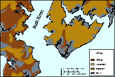
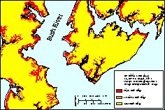
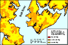
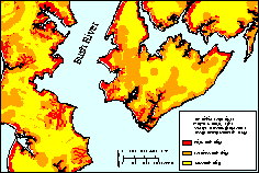
The percent occurrences of unique combinations of the four environmental variables were calculated for both the shell sites (Table 1) and the non-shell sites (Table 2). For example, in the shell data, 34.7% of the known sites are within 500 feet of brackish water, the nearest water type is brackish, the elevation is 20 feet or less, and the topography is a terrace or a bluff. Similar to logistic regression, the unique combination model design associated site potential with the occurrence of a unique combination of environmental factors. Instead of calculating a probability, however, it simply used the observed frequency of the unique combination as the measure of site potential. To locate cells with these unique combinations in the GIS, the Grid COMBINE function was used to produce a GIS layer with a value for each unique combination of the environmental variables. A high potential was assigned to unique combinations occurring over 20% of the time, medium potential to 6.25% to 20%, and low or no potential to less than 6.25%. (The eight combinations would each constitute 6.25% of the total if they were equal in distribution.) These site potential levels were linked to the grid value attribute table (VAT) using a relational join in the database. This procedure assigned the site potential to each cell in the map, and results could be queried and visualized. A layer showing the combined results of the shell and non-shell versions of the model was also produced with the Grid MAX function. Results of the shell, non-shell, and combined analyses are shown in Figures 11, 12, and 13, respectively, for a portion of the study area.
| Distance to water (ft) | Water type | Elevation (ft) | Topography | Frequency | Percentage |
| 0-500 | Brackish | 0-20 | Terrace/Bluff | 75 | 34.7 |
| 0-500 | Brackish | 0-20 | Floodplain/Flat | 81 | 37.5 |
| 0-500 | Brackish | > 20 | Terrace/Bluff | 14 | 6.5 |
| 0-500 | Brackish | > 20 | Floodplain/Flat | 2 | 0.9 |
| 0-500 | Fresh | 0-20 | Terrace/Bluff | 24 | 11.1 |
| 0-500 | Fresh | 0-20 | Floodplain/Flat | 10 | 4.6 |
| 0-500 | Fresh | > 20 | Terrace/Bluff | 4 | 0.9 |
| > 500 | Brackish | 0-20 | Terrace/Bluff | 4 | 1.9 |
| > 500 | Fresh | 0-20 | Terrace/Bluff | 2 | 0.9 |
| Totals | 216 | 100.0 | |||
| Distance to water (ft) | Water type | Elevation (ft) | Topography | Frequency | Percentage |
| 0-500 | Fresh | > 20 | Terrace/Bluff | 89 | 27.3 |
| 0-500 | Fresh | > 20 | Floodplain/Flat | 14 | 4.3 |
| 0-500 | Fresh | 0-20 | Terrace/Bluff | 27 | 8.3 |
| 0-500 | Fresh | 0-20 | Floodplain/Flat | 23 | 7.1 |
| 0-500 | Brackish | > 20 | Terrace/Bluff | 27 | 8.3 |
| 0-500 | Brackish | > 20 | Floodplain/Flat | 8 | 2.5 |
| 0-500 | Brackish | 0-20 | Terrace/Bluff | 33 | 10.1 |
| 0-500 | Brackish | 0-20 | Floodplain/Flat | 35 | 10.7 |
| > 500 | Fresh | > 20 | Terrace/Bluff | 26 | 8.0 |
| > 500 | Fresh | > 20 | Floodplain/Flat | 34 | 10.4 |
| > 500 | Fresh | 0-20 | Terrace/Bluff | 2 | 0.6 |
| > 500 | Fresh | 0-20 | Floodplain/Flat | 2 | 0.6 |
| > 500 | Brackish | > 20 | Terrace/Bluff | 2 | 0.6 |
| > 500 | Brackish | 0-20 | Terrace/Bluff | 4 | 1.2 |
| Totals | 326 | 100.0 | |||
RESULTS AND DISCUSSION
Several approaches were used to evaluate and validate the site potential maps, including calculating the percentage of the land area covered by each potential category, comparing the locations of known sites to the corresponding site potential, and calculating Kvamme's Gain Statistic (1 - [% area / % known sites]) (Kvamme 1988). Results are shown in Table 3. The shell site potential map corresponded well with known sites in the region. This correspondence can be attributed to several factors. The environmental characteristics associated with these sites are well defined, the model was focused specifically on these types of sites, and the mix of environmental conditions identified in the model development process matches well with shoreline surveys used to discover the sites. Results were less successful for the non-shell sites, although only one known site fell in a low potential area. Statistical factors leading to this lower result include competing variables in the less homogeneous grouping of non-shell sites and higher measures of association between the non-shell environmental variables. Also, APG has no known (recorded) non-coastal prehistoric sites, and very little of the interior has been intensively surveyed. Since interior surveys are more revalent in the regional data used to design the model, the model may be more useful than the validation suggests for indicating areas of high potential in the interior of the APG site. Results from interior surveys of the site would be invaluable for further evaluation and improvement of the model.
| Site potential | Percent of site area | Number of known sites | Kvamme's Gain Statistic | ||||||
| Shell | Non-shell | Combined | Shell | Non-shell | Combined | Shell | Non-shell | Combined | |
| High | 16.5 | 2.7 | 19.2 | 12 | 2 | 42 | 0.82 | 0.55 | 0.79 |
| Medium | 2.5 | 44.3 | 29.0 | 0 | 30 | 4 | 0.80 | 0.52 | 0.52 |
| Low | 81.0 | 53.0 | 51.8 | 1 | 1 | 0 | - | - | - |
Despite the limitations of this analysis and predictive archaeological modeling in general, the results of the study provide a useful map for refining and reducing areas of potential high probability for sites. Ground truthing is necessary to better validate the results. Modeling cannot take the place of intensive archaeological survey to discover sites, but it does provide planners with a guide showing areas that would likely require less time, effort, and money to develop from a cultural resources compliance standpoint. Priority areas for evaluation, monitoring, or mitigation are augmented by the model results.
As shown by this study, good results can be achieved from archaeological predictive modeling with available data even if the requirements for logistic regression cannot be met. In cases where predictive modeling (especially logistic regression) is planned or likely to occur, improved sampling and data collection procedures are likely to increase the efficiency and quality of modeling. Survey locations can be planned with statistically based methods to reduce bias and ensure that a representative set of unique environmental conditions is accounted for. Data collection procedures can be improved through systematic, quantitative, and thorough collection of information during surveys, including collection of data in locations surveyed where no sites were found.
ACKNOWLEDGMENTS
We would like to thank Reed MacMillian, David Blick, and other staff members of the Directorate of Safety, Health and Environment at Aberdeen Proving Ground for their support and encouragement during this project. Thanks also to John Hoffecker for his guidance and interest in the archaeological elements of this work, to Richard Olsen for his management support, John Krummel for his review of the initial draft of this document, and to Joan Meyer and Margaret Greaney for their GIS contributions. This project was sponsored by the U.S. Army as part of a larger environmental analysis for Aberdeen Proving Ground. This work was supported under a military interdepartmental purchase request from the U.S. Department of Defense, U.S. Army, through U.S. Department of Energy contract W-31-109-Eng-38.
DISTRIBUTION STATEMENT AND DISCLAIMER
Distribution restriction statement: Approved for public release: Distribution is unlimited. #3159-A-5
Neither the U.S. Army, nor any of its employees or officers, makes any warranty, express or implied, or assumes any legal liability or responsibility for the accuracy, completeness, or usefulness of any information, apparatus, product, or process disclosed, or represents that its use would not infringe privately owned rights.
Reference to any specific commercial product, process, or service by trade name, trademark, manufacturer, or otherwise does not necessarily constitute or imply its endorsement, recommendation, or favoring by the U.S. Army. The views and opinions of the authors do not necessarily state or reflect those of the U.S. Army.
Directorate of Safety, Health and Environment (DSHE), 1996, Geographic Information System database, U.S. Army, Aberdeen Proving Ground, MD.
BRW, Inc., 1996, Draft Research Design for the Development of a High Probability Predictive Model for Identifying Archaeological Sites, prepared for Minnesota Department of Transportation, Saint Paul, MN.
Kuiper, J.A., 1996, Producing a Programmatic Environmental Impact Statement for a Large Federal Facility: A GIS Technical Leader's Perspective, paper presented at the 16th Annual Esri User Conference, Palm Springs, CA.
Kvamme, K., 1988, Development and testing of quantitative models. In W.J. Judge and L. Sebastian (eds), Quantifying the Present and Predicting the Past: Theory, Method, and Application of Archaeological Predictive Modeling, U.S. Department of the Interior, Bureau of Land Management Service Center, Denver, CO, pp. 325 - 428.
Maryland Historical Trust (MHT), 1995, Maryland archaeological site files and maps, Crownsville, MD.
SAS Institute, Inc., 1990, The CATMOD Procedure - Cautions. In SAS/STAT User's Guide, Version 6, Fourth Edition, Volume 1, Cary, NC, pp. 462-463.
Wescott, K.L., and J.A. Kuiper, 1999, Using a GIS to Model Prehistoric Site Distributions in the Upper Chesapeake Bay. In K.L. Wescott and R.J Brandon (eds), Practical Applications of GIS for Archaeologists: A Predictive Modeling Tool-Kit. London: Taylor & Francis (in press).
AUTHOR INFORMATION
James A. Kuiper (jkuiper@anl.gov): Biogeographer / GIS Analyst