Gordon Wells
PR Blackwell
Precision Image Mapping: Georeferenced Imagery
Produced from High-Resolution
Orthoimages
Abstract
With the growing availability of orthoimages, the possibility now exists to produce image maps
from aerial photographs for areas of low and moderate relief. Experiments in Texas using
photographs acquired after the release of Texas Orthoimagery Program (TOP) products have
generated image maps with a horizontal precision of better than 10 meters for areas having up to
70 meters of vertical relief. Without resorting to full orthoimage production requiring topographic
scaling, camera system metrics, and other information, precision image maps at a scale of
1:12,000 can be derived using TOP orthoimages for control. The technique holds promise for
rapid image map generation for emergency response and for historical image maps showing the
changing Texas landscape.
Introduction
Through the National Digital Orthophotography Program and many state- and locally-funded efforts, high-resolution orthoimagery at scales of 1:24,000 to 1:1200 is becoming available in the public domain for many regions of the USA. In Texas, the Strategic Mapping Program (StratMap) coordinates the production of 1-meter, 24-bit color infrared digital orthoimages at a scale of 1:12,000 for the entire state. As the program reaches completion in the year 2000, this state resource of more than 17,000 quarter-quadrangle orthoimages will provide new opportunities to develop more accurate GIS data in both the government and private sectors. Additional opportunities are now emerging to apply non-traditional techniques to the production of the next generation of rectified, georeferenced imagery.
Rectification Techniques
Several methodologies can be applied to the rectification and georegistration of digitized aerial photographs. The techniques fall into three categories:
1) Differential rectification by spatial resection
The production of conventional digital orthoimagery involves the establishment of interior orientation for the scanned photograph, including location of the principal point, fiducial measurements, reference to the camera metrics report and creation of an image coordinate system. Next, the image is correlated to a ground coordinate system through the establishment of exterior orientation, which accounts for platform rotation angles, produces colinearity equations and generates real-world coordinates for the location of picture elements. High-precision field surveys are performed to collect control points, and the set of control points is densified through the process of fully analytical aerial triangulation. Once established, these elements are combined with a digital elevation model of the terrain to produce high-resolution orthoimages that often exceed National Map Accuracy Standards (NMAS) for 1:12,000 scale, which confine errors in horizontal location to less than 10 meters. Whereas differential rectification by spatial resection is the most accurate technique available for the production of georeferenced imagery, it is also the most expensive and makes the most demands upon the technical management of large projects.
2) 2nd- to nth-order nonlinear rectification (rubber sheeting)
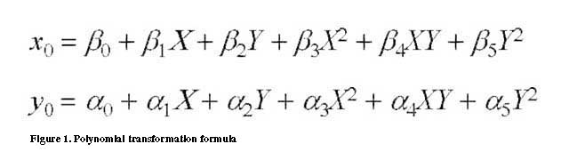
The primary technique under consideration in this paper involves the use of polynomials in the transformation of picture element locations. The process uses a source image, such as an existing orthoimage, or a vector file, such as a road system with intersections, or a matrix of photo-identifiable points that are mapped to a real-world coordinate system. A destination image of the scanned aerial photograph is then rectified by polynomial transformation to match ground control points selected from the source data. For aerial photographs, a polynomial transformation of 3rd (or greater) order is required to remove most image distortions. The equations representing polynomial transformation can be expressed as shown in Figure 1.
 Rectification techniques that rely upon polynomial transformations are often called rubber sheeting and have been in use for many years. They are simple to employ and produce rapid results. The major drawbacks of the techniques have been their inconsistency and lack of horizontal accuracy, when compared to the results obtained by traditional orthoimage production by spatial resection.
3) Terrain-corrected nonlinear rectification
Research has recently focused attention on other methods of image rectification that do not require the many elements of differential rectification, but do account for relief displacement by incorporating a digital elevation model (DEM). Ordinary kriging algorithms can be adapted to include data derived from a DEM to remove spatial distortions in aerial images (Ke-Sheng et al. 1999). Direct linear transformation also includes digital terrain data in a manner similar to differential rectification, but eliminates the necessity for fiducial measurements, platform orientation and camera calibration in the creation of rectified, georeferenced imagery (Butler and Carson 1999). Techniques of this kind need to be further investigated to assess their efficiency and accuracy.
Horizontal Accuracy of Texas Orthoimagery Program DOQs
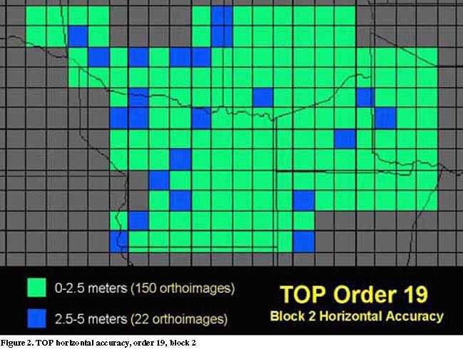
In Texas, the 1-meter color infrared orthoimages created by the Texas Orthoimagery Program (TOP) component of StratMap are closely checked for their positional accuracy at several stages of the production process. In addition to field survey points collected with high-precision GPS instruments for use in differential rectification by commercial orthoimagery firms, quality assurance points are gathered that are never supplied to the contractors. These survey control points can be used to assess the horizontal accuracy of finished orthoimages delivered to the state. Contracts with the firms specify that any quarter-quadrangle orthoimages having features displaced by more than ten meters from their locations established by precision GPS instruments must be replaced. In practice, the orthoimagery produced under TOP has attained a much higher level of horizontal accuracy than merely meeting the National Map Accuracy Standards for 1:12,000 scale. Measured horizontal offsets are less than 5 meters for most all products and less than 2.5 meters over broad areas (Figure 2).
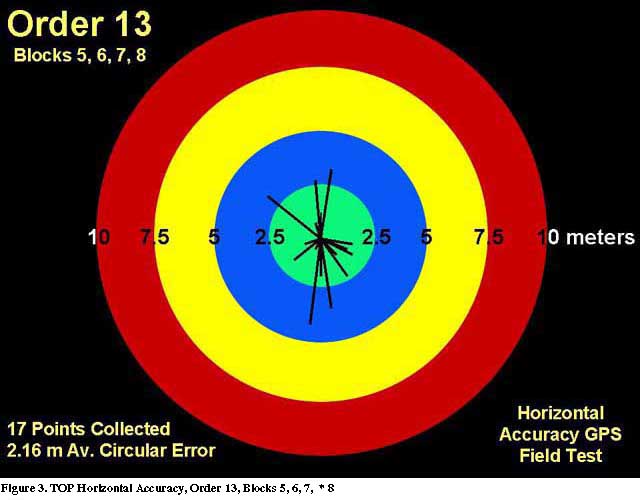
 In regions where possible discrepancies may have occurred during the production process, new GPS surveys are performed after the completion of orthoimagery. Most of the validation surveys have uncovered no problems and can be used as further illustration of the accuracy of the TOP orthoimages (Figure 3).
Precision Image Mapping in East Texas
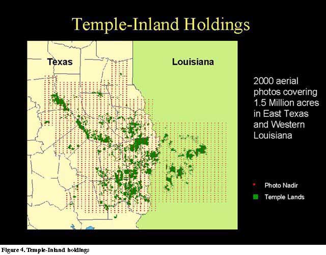
Temple-Inland (TI) owns approximately 1.5 million acres of forestland in eastern Texas and western Louisiana. (Figure 4). In late-1998, TI contracted with Aerial Data Services of Tulsa, Oklahoma, to acquire color infrared photography coverage for their entire land holdings. The aerial survey was completed in the winter of 1999, and the Forest Resources Institute was contacted concerning the production of rectified, georeferenced imagery for the large collection of aerial photographs.
 Plans were initially made to use TI's SPOT satellite imagery to rectify and georegister the imagery. However, as the project was being planned, StratMap's Texas Orthoimagery Program began to deliver DOQ imagery for East Texas. The TOP orthoimages represented an exceptionally accurate, high-resolution base for rectifying the TI aerial photography. To determine the feasibility of such an approach, a pilot project was conducted using the TOP DOQs. Successful results obtained from initial tests were sufficient to justify continuation of the project using TOP DOQs wherever possible.
Methodology
The production procedure developed during the pilot project consists of the following basic steps:
1. Aerial photographs are scanned to provide coverage of a complete 7.5-minute USGS quadrangle.
2. A base map mosaic is constructed from TOP DOQ quarter-quads sufficient to contain the area of each aerial photograph.
3. 25 Ground Control Points (GCPs) are selected at locations equally distributed across each aerial image and the DOQ.
4. 3rd-Order polynomial transformation is used to "rubber-sheet" the image.
5. The rectified image is checked for horizontal accuracy (less than 10 meter offset from features in the DOQ).
6. Images are mosaicked to conform to the area of a 7.5-minute quad (Normally, eight to twelve images are required.).
7. The Image mosaic is clipped to 7.5-minute quadrangle boundaries and subset for distribution.
8. Final QA/QC is performed by spot checking against common features identified in the DOQ base.
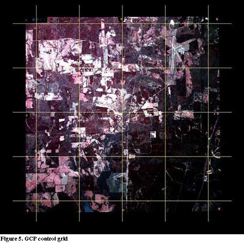
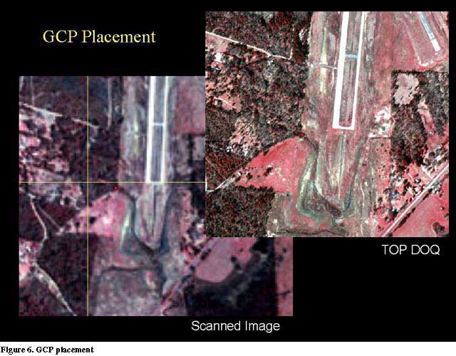
A uniform distribution of GCPs is extremely important to achieve maximum horizontal accuracy with a minimum number of control points. In order to assist placement of GCPs, a control grid is superimposed on the imagery (Figure 5). GCPs are selected as close as possible to the grid intersections. Even in those cases where more easily distinguished points are available, preference is given to points closer to the target coordinates (Figure 6).
In cases where no identifiable GCPs are possible at the desired coordinates, interpolated points are added using the "predict" function available in most image processing software. Although such points do nothing to improve the fit of the transformation, adding them prevents the introduction of distortion caused by an uneven distribution of control points.
Selecting GCPs at this density within a restricted distribution pattern is demanding. New technicians require a degree of training and experience to become proficient. However, most are able to gain the required proficiency within a few weeks. Technicians work on entire quadrangles independently, though they commonly assist each other on particularly difficult images. Informal meetings are held frequently to discuss issues and share ideas.
Accuracy Assessment
As work progressed, it became evident that the image mapping program was exceeding expectations in terms of the horizontal accuracy attained. To quantify the results, a rigorous accuracy assessment was undertaken in Nacogdoches County, Texas. The Nacogdoches South NE quarter-quad was selected because of it's proximity to the Forest Resources Institute and because it offered the type of rolling topography which had proven well-suited to the precision image mapping techniques in use (Figure 7).
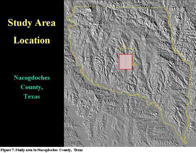 The topography of the study area ranges from approximately 70 to 143 meters in elevation, with over 70 meters of vertical relief consisting of moderate, rolling terrain. The selected area contains the southwestern portion of the City of Nacogdoches, Texas, thus affording many opportunities to locate easily identifiable and accessible features for horizontal accuracy assessment.
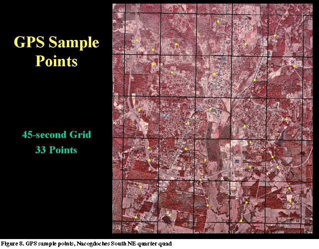
The Nacogdoches South NE quarter-quad was divided into 25 separate 45-arc-second segments. Within each segment, control points were selected at random intervals (Figure 8). Criteria for selection included the ability to locate the point on the DOQ, the ability to locate the point on the image mapping product and accessibility on the ground. Each point was plotted against the DOQ base map as a point feature in an Esri shapefile.
The topography of the study area ranges from approximately 70 to 143 meters in elevation, with over 70 meters of vertical relief consisting of moderate, rolling terrain. The selected area contains the southwestern portion of the City of Nacogdoches, Texas, thus affording many opportunities to locate easily identifiable and accessible features for horizontal accuracy assessment.
The Nacogdoches South NE quarter-quad was divided into 25 separate 45-arc-second segments. Within each segment, control points were selected at random intervals (Figure 8). Criteria for selection included the ability to locate the point on the DOQ, the ability to locate the point on the image mapping product and accessibility on the ground. Each point was plotted against the DOQ base map as a point feature in an Esri shapefile.
 Field data were collected using a Trimble Pro XRS GPS receiver. Both real-time and post processing differential correction were applied to achieve a horizontal accuracy of 1 meter at the 95 percent confidence level. The GPS points were exported in Esri shapefile format. Five observers were then asked to locate the control points on each of three precision image map products. These three mosaicked images were the results of three separate applications of precision image mapping procedures applied to the same set of imagery. Each observer's points on each of the three samples were stored in separate shapefiles. Figure 9 illustrates three points (GPS, DOQ, target) generated by each observer for each control point on each sample.
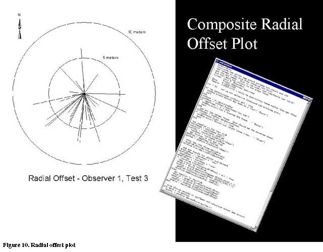
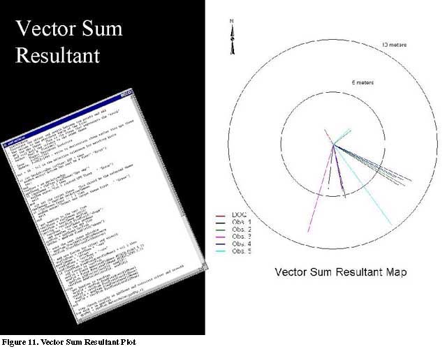
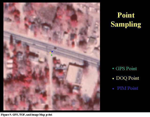 Avenue code was written to analyze the magnitude and direction of the offset of the DOQ and target points from the field surveyed (GPS) location (Appendix I). The offset and azimuth were written as attributes to the target point shapefile by the Avenue code. Avenue was also used to plot the radial offset of each control point (Figure 10). Each vector in the composite radial offset plot represents the direction and magnitude of the offset of one control point. A vector sum resultant plot was also generated using Avenue (Figure 11). This plot shows the overall error magnitude and direction for all points collected by one observer on one sample.
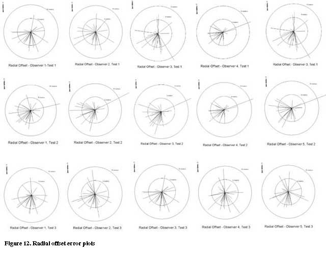
 The plots indicate that the range of error falls well within the 10-meter limit imposed by National Map Accuracy Standards for 1:12,000 scale. Figure 12 contains composite radial offset plots for each sample and observer for all cases. Rows represent samples, and columns, observers. Note that all samples and all observers show similar offset direction and magnitude patterns. The slight southeast bias of the errors is also reflected in the DOQ radial offset plot. Sample 2 indicates one point beyond the 10-meter limit recorded by all observers. This anomaly represents an error in the rectification applied to one of the images in Sample 2 during the image mapping process.
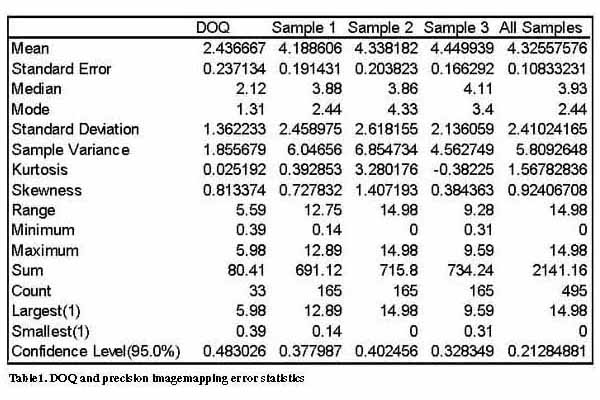
Statistical Analyses
Statistical analyses of these results are given in Table 1. For the test in Nacogdoches South NE, the average DOQ offset was 2.4-meters with a standard error of 0.24. The average offset of all precision image mapping samples was 4.3-meters with a standard error of 0.11. The results are well within National Map Accuracy Standards for a scale of 1:12,000.
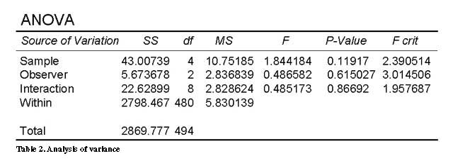
To determine the effects of human interaction in the accuracy assessment process, a two-way analysis of variance with replication was performed. The results are given in Table 2. These data indicate that neither observers nor samples were a significant source of variation in the test data.
Limitations of Precision Image Mapping
Precision image mapping has been shown to be an effective and highly accurate method to obtain georeferenced imagery in areas of moderately rolling topography. One should be aware, however, that there exist several limitations to the process. First is the requirement for highly accurate digital orthoimagery to serve as control. Our analysis demonstrates that the maximum accuracy possible using precision image mapping is approximately one-half that of the base data. If the base orthoimagery falls at the limit of acceptable horizontal error, then any image map products based on that orthoimagery will likely fail to meet National Map Accuracy Standards.
There are terrain limitations as well. Figure 13 illustrates several conditions that serve to limit accuracy. In East Texas, it is not unusual to find large areas of homogeneous, undisturbed vegetation. These pose a serious problem for identifying ground control points. In some cases it is possible to identify particularly prominent tree crowns or other natural features. Care must be exercised, however, to avoid errors introduced by sun angle, natural disturbances or image layover of features photographed at a distance from the principal point of the frame. Large water bodies offer a similar challenge. The choice then lies between selecting a point far from the desired location or predicting a point within the inundated area.
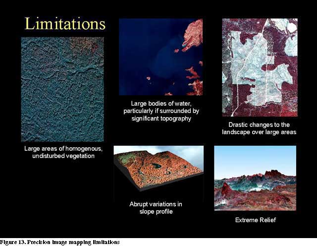 Areas that have suffered drastic changes since the DOQ was acquired also present significant difficulties. Clearcuts and forest fires often leave no identifiable features in their wake. If these disturbances cover significant areas, they can drastically affect the accuracy of the polynomial transformation.
Abrupt variations in slope profile create pockets of error in the vicinity of the variations and sometimes systematically across larger areas of the image. Adding additional GCPs along both sides of the feature sometimes helps. In this case, care is required to avoid adversely weighting the polynomial solution.
Finally, areas of extreme topographic variation, such as mountainous regions, may present unavoidable and unresolvable difficulties for this process.
Areas that have suffered drastic changes since the DOQ was acquired also present significant difficulties. Clearcuts and forest fires often leave no identifiable features in their wake. If these disturbances cover significant areas, they can drastically affect the accuracy of the polynomial transformation.
Abrupt variations in slope profile create pockets of error in the vicinity of the variations and sometimes systematically across larger areas of the image. Adding additional GCPs along both sides of the feature sometimes helps. In this case, care is required to avoid adversely weighting the polynomial solution.
Finally, areas of extreme topographic variation, such as mountainous regions, may present unavoidable and unresolvable difficulties for this process.
Future Tests
A series of future tests of the horizontal accuracy of precision image mapping is planned to determine the suitability of the procedures in areas of greater topographic relief and variation. Tests will be conducted in the steep-slope terrain of the central Texas Hill Country and in the mountainous region of West Texas. The future studies will determine if precision image mapping can contribute to the production of rectified, georeferenced imagery in other parts of the state where topographic relief is less uniform.
Implications for StratMap2
The methodology discussed in our paper already holds considerable promise for future applications in the state of Texas. As StratMap2 funds are secured for the replacement of TOP orthoimagery following the 2001/2002 cycle of National Aerial Photography Program data collection, precision image mapping products can be created for large parts of the low-relief areas of the state at a small fraction of the cost of differential rectification by spatial resection. The image maps would maintain National Map Accuracy Standards for a scale of 1:12,000, and the resulting savings could be spent to purchase higher resolution orthoimagery for areas of rapid change and other special interest.
Another immediate use for precision image mapping products would benefit emergency response activities. In the days following natural or man-made disasters, such as floods, tornadoes, fires and oil spills, federal, state and private organizations often collect aerial photographs of the affected areas. Although these uncorrected aerial images are useful as photointerpretive tools for damage assessment, they offer limited value for GIS studies. Precision image mapping products generated rapidly (perhaps within 24 hours) after these aerial photographic surveys could aid field teams equipped with GPS instruments and laptop and pen-based computers. Reconnaissance teams could map and annotate their field studies using actual images of the results of the disaster.
Just as the TOP DOQs can provide a source for control to make precision image maps from future aerial photography, the same orthoimagery can be used to rectify and georeference historical aerial photographs. As state archives of aerial photographs are converted to digital format for long-term preservation, retrospective image mapping products of great interest and value can be created for areas of Texas that have undergone significant landscape changes since the 1930s.
Each of the above applications of precision image mapping is considered important to the success of the next round of statewide digital base map development to be conducted during StratMap2.
References
Butler, B.J. and W.W. Carson (1999) Assessment of differential, direct linear transformation, and rubbersheeting techniques for rectifying digital aerial photographs. ASPRS 1999 Annual Conference Proceedings. 911-17.
Ke-Sheng Cheng, Chang-Hsuan Tsai, Hui-Chung Yeh and I. Hueter (1999) A new approach to image rectification by kriging. ASPRS 1999 Annual Conference Proceedings. 783-89.
Tables
Acknowledgements
The Forest Resources Institute (FRI) Precision Image Mapping (PIM) project would not be possible without the dedication and diligence of the Institute's students and staff. Under the direction of Mr. Blackwell, the FRI PIM team perfected the precision image mapping procedures presented in this paper and carried out the accuracy assessment. The team consists of the following individuals:
Qinghou Li, Project Lead
Katie Springer, Research Associate, GIS
Dana Beck, GIS Assistant
Byron Kilburn, GIS Assistant
Appendix
Avenue Code Listings
PIMCalcError.ave
' NAME: PIMCalcError
' DESC: Calculate the offset and azimuth between two points and add
'       the values to the attribute table of the first
' AUTH: Paul R. Blackwell
'       Forest Resources Institute
'       Stephen F. Austin State University
' Date: 6-JULY-1999
' Update:7-JULY-1999 - write to destination theme rather than gps theme

tol = 50 ' tol is the selection tolerance for matching points

if (av.GetActiveDoc.is(View).NOT ) then
  msgBox.error("Active Doc must be a View!","Error")
  exit
end
theView = av.getActiveDoc
gpsTheme = theView.FindTheme("Gps.shp")
if (gpsTheme = -1 ) then
  msgBox.error("Can't located GPS Theme...","Error")
  exit
end
' now get the target theme.  This should be the selected theme
theThemes = theView.GetActiveThemes
if (theThemes.Count <> 1 ) then
  msgBox.error("Select one target theme first...","Error")
  exit
end

'get handles to the test ftab
testTheme = theThemes.get(0)
testFtab = testTheme.getFtab
testShp = testFtab.FindField("shape")
' testName = testTheme.getName
' get handles to the gps ftab
gpsFtab = gpsTheme.GetFtab
gpsShp = gpsFtab.FindField("shape")

' make the test theme editable
' gpsFtab.StartEditingWithRecovery
testFtab.StartEditingWithRecovery

' add new fields for offset and azimuth
'errFldName = testName + "-err"
errFldName = "offset"
'azmFldName = testName + "-azm"
azmFldName = "azimuth"
if (testFtab.FindField(errFldName) = nil ) then
  'add fields to testFtab
  errFld = Field.Make(errFldName,#FIELD_FLOAT,5,2)
  azmFld = Field.Make(azmFldName,#FIELD_LONG,5,0)
  'gpsFtab.AddFields({errFld, azmFld})
  testFtab.AddFields({errFld, azmFld})
else
  'get handles to testFtab
  'errFld = gpsFtab.FindField(errFldName)
  errFld = testFtab.FindField(errFldName)
  'azmFld = gepFtab.FindField(azmFldName)
  azmFld = testFtab.FindField(azmFldName)
end

' step throuh records in gpsTheme and calculate offset and azimuth
for each r in gpsFtab
  gpsPnt = gpsFtab.ReturnValue(gpsShp,r)
  ' find the closest point in the test theme
  testFtab.SelectByPoint(gpsPnt,tol,#VTAB_SELTYPE_NEW)
  testSel = testFtab.GetSelection
  if (testSel.Count <> 1 ) then
    offset = 9999
    azm = 9999
  else
    for each p in testSel
      testPnt = testFtab.ReturnValue(testShp,p)
      offset = gpsPnt.distance(testPnt)
      gpsVector = PointZ.Make(gpsPnt.getX, gpsPnt.getY,0)
      testVector = PointZ.Make(testPnt.getX, testPnt.getY,0)
      'azm = vector.Difference(testVector,gpsVector)
      azm = vector.Difference(gpsVector,testVector)
      'gpsFtab.setValueNumber(errFld,r,offset)
      testFtab.setValueNumber(errFld,p,offset)
      'gpsFtab.setValueNumber(azmFld,r,azm.GetAzimuth)
      testFtab.setValueNumber(azmFld,p,azm.getAzimuth)
    end
  end
end

'stop the edit session
testFtab.StopEditingWithRecovery(True)
PIMRadialPlot.ave
' NAME: PIMRadialPlot.ave
' DESC: plots offset and azimuth fields in a vtab as a radial plot
'
' AUTH: Paul R. Blackwell
'       Forest Resourcs Institute
' DATE:   06-JULY-1999
' HIST:
'
'get a value for the plot maginfication
mag = msgBox.input("Enter Maginfication Factor","Magification","100").asNumber

' make sure active doc is a view
if (av.GetActiveDoc.is(View).NOT ) then
  msgBox.error("Active Doc must be a View!","Error")
  exit
end
theView = av.getActiveDoc

' generate a line symbol
vectorSym = symbol.Make(#SYMBOL_PEN)
vectorSym.SetSize(1)
vectorSym.setColor(color.GetRed)

' the source theme should be the active theme
theThemes= theView.GetActiveThemes
if (theThemes.count <> 1) then
  msgBox.err("Select 1 and only 1 theme first","Error")
  exit
end
srcTheme = theThemes.Get(0)

' get handles for the src theme
srcFtab = srcTheme.GetFtab
errFld = srcFtab.FindField("offset")
azmFld = srcFtab.FindField("azimuth")

' find the origin for the plot
srcDisplay = theView.GetDisplay
srcGraphics = theview.GetGraphics
origin = srcDisplay.ReturnExtent.returnCenter

' draw scale
c5 = Circle.Make(origin,5 * mag)
c10 = circle.make(origin,10 * mag)
graphicC5 = graphicShape.make(c5)
graphicC10 = graphicShape.make(c10)

srcGraphics.add(graphicC5)
srcGraphics.add(graphicC10)

' now draw the vectors
for each r in srcFtab
  offset = srcFtab.returnValueNumber(errFld,r)
  azimuth = srcFtab.returnValueNumber(azmFld,r)
  'modify azimuth to change origin and direction
  azimuth = azimuth + 90
  if (azimuth > 360) then
    azimuth = azimuth - 360
  end
  azimuth = 360 - azimuth
  if (offset <> 0 ) then
    xoffset = azimuth.asRadians.cos * offset * mag
    yoffset = azimuth.asRadians.sin * offset * mag
    endPnt = point.Make( origin.GetX  + xoffset, origin.GetY + yoffset)
    theLine = Line.Make(origin,endPnt)
    theGraphicLine = graphicShape.Make(theLine)
    srcGraphics.Add(theGraphicLine)
  end
end
PIMVectRest.ave
' NAME: PIMVectRest.ave
' DESC: plots the vector resultant for all themes in the view
'
' AUTH: Paul R. Blackwell
'         Forest Resourcs Institute
' DATE:   15-JULY-1999
' HIST:
'
'get a value for the plot maginfication
mag = msgBox.input("Enter Maginfication Factor","Magification","100").asNumber

' make sure active doc is a view
if (av.GetActiveDoc.is(View).NOT ) then
  msgBox.error("Active Doc must be a View!","Error")
  exit
end
theView = av.getActiveDoc

' find the origin for the plot
srcDisplay = theView.GetDisplay
srcGraphics = theview.GetGraphics
origin = srcDisplay.ReturnExtent.returnCenter

' remove any old graphics
srcGraphics.empty

' draw scale
c5 = Circle.Make(origin,5 * mag)
c10 = circle.make(origin,10 * mag)
graphicC5 = graphicShape.make(c5)
graphicC10 = graphicShape.make(c10)
srcGraphics.add(graphicC5)
srcGraphics.add(graphicC10)

theThemes= theView.GetThemes
if (theThemes.count < 1) then
  msgBox.err("Must have more than 1 theme","Error")
  exit
end

' repeat this for each theme in the view
for each srcTheme in theThemes

  ' get handles for the src theme
  srcFtab = srcTheme.GetFtab
  errFld = srcFtab.FindField("offset")
  azmFld = srcFtab.FindField("azimuth")

  ' get the symbol color for this theme
  theLegend = srcTheme.getLegend
  theColor = theLegend.getSymbol(theLegend.ReturnFieldNames, False).GetColor

  ' calculate the resultant the vector
  for each r in srcFtab
    offset = srcFtab.returnValueNumber(errFld,r)
    azimuth = srcFtab.returnValueNumber(azmFld,r)
    'modify azimuth to change origin and direction
    azimuth = azimuth + 90
    if (azimuth > 360) then
      azimuth = azimuth - 360
    end
    azimuth = 360 - azimuth
    start = origin
    if (offset <> 0 ) then
      xoffset = azimuth.asRadians.cos * offset * mag
      yoffset = azimuth.asRadians.sin * offset * mag
      endPnt = point.Make( start.GetX  + xoffset, start.GetY + yoffset)
      theLine = Line.Make(start,endPnt)
      start = endPnt
    end
  end

  ' draw the resultant vector
  theLine = Line.Make(origin,endPnt)
  theGraphicLine = graphicShape.Make(theLine)
  theSym = symbol.Make(#SYMBOL_PEN)
  theSym.setColor(theColor)
  theGraphicLine.setSymbol(theSym)
  srcGraphics.Add(theGraphicLine)
end