PR Blackwell
Gordon Wells
DEM Resolution and Improved Surface Representation
Abstract
Digital elevation models (DEMs) are increasingly employed for orthoimagery production, hydrologic modeling, view-shed determination, slope/aspect analyses, and three-dimensional surface visualization. DEMs in common use range from relatively coarse three-arc-second (100-meter profile) Level 1 DTEDs to 30-meter profile Level 2 DEMs produced by the U.S. Geological Survey. Yet these data sets may not capture sufficient surface detail to meet the requirements of many applications. Experiments in Texas involving a variety of terrain types demonstrate the effectiveness of higher resolution DEMs, especially 10-meter profile data sets, in the creation of more geomorphologically accurate surface representations.
Introduction
GIS and image processing applications are making more frequent use of digital elevation models (DEMs) to represent landform features. Questions arise concerning the horizontal and vertical accuracy of DEMs from various sources created by different methodologies and their use for modeling natural processes, such as the simulation of drainage networks in hydrologic models. Our paper addresses several of these issues concerning DEM resolution and the accuracy of surface models.
Since the late-1980s, Level 1 Digital Terrain Elevation Models (DTED1) have been available for the USA. Prepared by the Defense Mapping Agency from USGS 1:250,000 scale 1 x 2-degree topographic sheets, the DTED1 data have a vertical accuracy of approximately 30 meters and horizontal profile of 3-arc-seconds, or approximately 100 meters. As coarse representations of broad-scale surface relief, DTED1 data is used for generalized models of entire river basins and as surfaces upon which to drape satellite imagery.
Beginning in the 1970s, the USGS produced 30-meter profile Level 1 DEMs using manual stereoplotters. Released in units of 7.5-minute quadrangles, the 30-meter Level 1 DEMs have a vertical accuracy of approximately 7 meters. Unfortunately, the Level 1 DEMs suffer from a wide variety of artifacts, including serious edgematching errors, striping and other anomalies. In recent years, the USGS has released 30-meter profile Level 2 products that are derived from the digital extraction of elevation data from the hypsography contour separates used in the production 7.5-minute topographic quadrangle maps. Whereas the horizontal profile remains the same as Level 1 products, vertical accuracy improves to within one-half contour interval of the source map, which lies in the range of 1 to 3 meters, except in mountainous terrain. Modelers have rapidly adopted the 30-meter Level 2 USGS DEM as the mainstay of many applications, especially slope/aspect and view-shed analysis and hydrologic modeling.
Over the past several months, a team of elevation scientists led by Susan Greenlee at the USGS EROS Data Center has made a great contribution to the community of DEM users by issuing sections of the National Elevation Dataset (NED), a seamless DEM tiled by one-degree blocks for regions of the conterminous USA. The NED contains edgematched Level 2 and Level 1 DEMs that have been filtered to remove their most serious flaws. Complete NED coverage for Texas has been available since the winter of 1999 and is already being used for watershed delineation and other GIS applications by several groups.
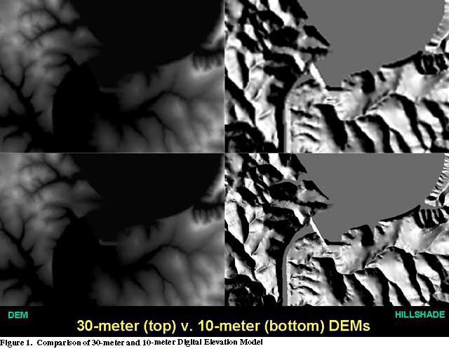
Still higher resolution DEMs are now in production for areas requiring more detailed surface models. Of particular interest are 10-meter drainage-enforced DEMs compiled using both the hypsography contour and hydrography elements present in 7.5-minute topographic quadrangle maps. 10-meter DEMs have the same vertical accuracy as 30-meter Level 2 products, but their 1/3-arc-second profile supplies a much improved representation of features of the actual landscape. The hillshade in Figure 1 illustrates the quality improvement gained by the 10-meter profile drainage-enforced DEM for an area of the Mansfield Dam 7.5-minute quadrangle in central Texas. Note the greater detail visible in the area of the dam and along minor drainages.
Surface Representation for Hydrologic Modeling
One test of the realism of digital elevation models is their capability to reflect the geomorphological qualities of common landforms. For many landforms, the measure of their representation in three dimensions can be a rather subjective judgment that lacks methods for exacting comparison. By contrast, hydrographic features represented in hydrologic models can be closely examined with respect to how well they capture important elements of geomorphological features that occur in the real landscape. For this assessment, an analysis of artificial flow paths was preformed using DEMs having various horizontal and vertical resolutions to determine their suitability for hydrologic modeling in selected study areas.
The hydrologic modeling was performed using ArcView Spatial Analyst. Because certain hydrologic functions are not supported in the ArcView user interface, basic Avenue code was written to complete the analysis (See Appendix). The feature analyzed was the artificial flow path calculated from each DEM. To generate flow paths in this manner, it is crucial to remove sinks occurring in the source elevation data. A sink is defined as a point into which all surrounding points flow, but flows into no other point. In other words, a cell in the DEM that is lower than all surrounding cells.
Spatial Analyst contains sample code that performs the task of filling the sinks that disrupt DEM surfaces using an Avenue program called Spatial.DEMFill. Spatial.DEMFill is run on the source DEM to produce a modified, sinkless surface. The resulting DEM is used as the input to the HydroFuntions script. The script calculates a FlowDirection theme and uses that result to calculate a FlowAccumulation theme. (Other functions in the script, watershed and sink, are not used to create artificial flow paths and are included for other purposes, such as the delineation of drainage basins.)
The FlowAccumulation theme consists of a raster where the value of each pixel represents the total number of pixels that flow into it. By selecting a threshold for the minimum number of pixels representing a drainage channel, an artificial flow path is generated. Symbology can then be used to designate stream order within a flow path. To maintain clarity in our graphics, no stream order symbolism was used for this analysis.
Examples from Austin, Texas
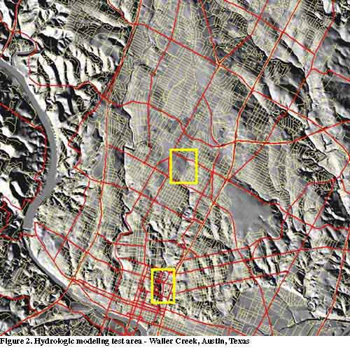
The climate and landscape of the Hill Country of central Texas make the region vulnerable to catastrophic flooding (Figure 2). Austin, the rapidly growing capital of Texas, lies along the eastern margin of the Hill Country and has experienced several disasterous floods in the past century. In 1981, a flashflood coursing down Shoal Creek near downtown Austin killed 13 people and caused more than $30 million in damage. The likely recurrence of flashfloods in urban Austin makes it important to create accurate landform representations from DEMs for use in hydrologic models.
Lower Waller Creek Watershed
The Waller Creek watershed lies entirely within the city limits of Austin, and its constricted valley surrounded by large areas of impermeable surface cover poses a serious threat for flooding. Figure 3 depicts the results of artificial flow path generation for the Lower Waller Creek study area. The lefthand image was generated using a standard 30-meter USGS Level 2 DEM. The righthand image employed a 10-meter profile drainage-enforced DEM shown in red and a 10-meter profile non-enforced DEM shown in yellow. The calculated 30-meter course generally flows within the valley, but deviates substantially from the actual channel location shown in black. The 10-meter profile DEMs produce much more realistic flow paths that correspond to the channel as it is mapped on the Austin East 7.5-minute USGS topographic quadrangle.
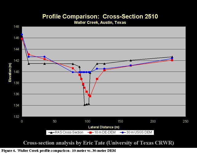
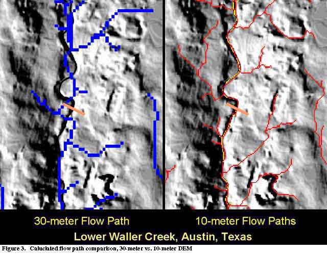 Figure 4 portrays an engineering cross-section profile near the 15th Street bridge crossing Waller Creek as indicated in Figure 3. The profile analysis was conducted by Eric Tate of the University of Texas Center for Research in Water Resources, and clearly demonstrates the superiority of a 10-meter drainage-enforced DEM developed by AverStar, Inc., over the standard 30-meter surface model. In this case, the 30-meter DEM fails to reflect any evidence of the stream channel.
Upper Waller Creek Watershed
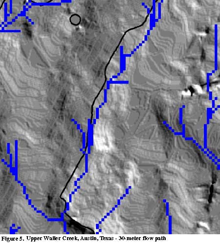
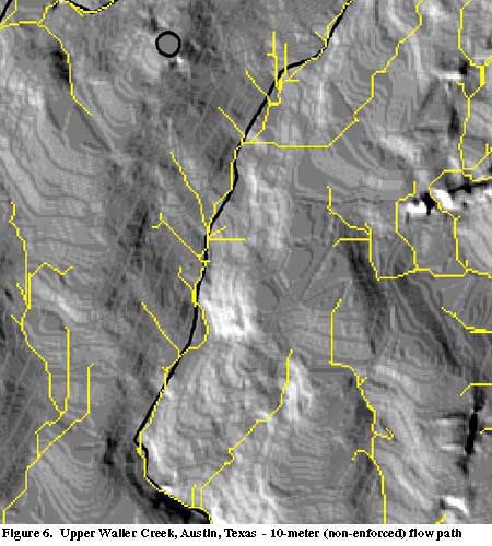
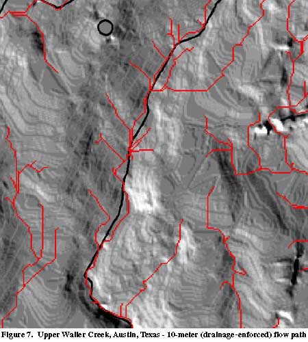
The Upper Waller Creek study area presents greater challenges for the modeler. Here the topographic variation is less pronounced, and the 30-meter DEM is capable of only very general indications of the stream course (Figure 5). The artificial flow path generated using the 10-meter non-enforced DEM provides a better representation of the stream, but fails to conform to the actual channel location in several segments (Figure 6). The 10-meter drainage-enforced DEM provides the best overall result, but its flow path also deviates slightly from the mapped channel location in several places (Figure 7). In general, 10-meter DEMs, especially those created with enforced drainage, appear to provide excellent surfaces for use in hydrologic models of drainage across landscapes containing moderate relief.
Examples from Houston, Texas
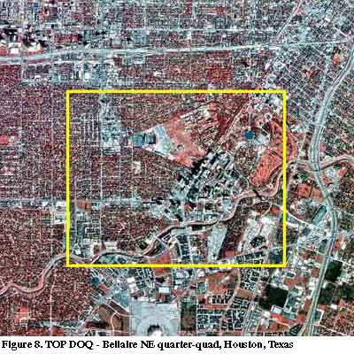
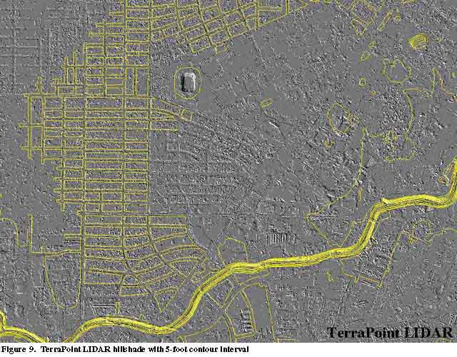
We have seen in the examples above that reduction in topographic relief can limit the accuracy of digital surface representations for drainage features. But what about extremely flat terrain? A Texas Orthoimagery Program DOQ of the Bellaire NE quarter-quad in Houston (Figure 8) shows West University Place and the campus of Rice University near Brays Bayou. The area is extremely flat and subject to frequent flooding. 5-foot contour intervals draped over a hillshade made from 1-meter TerraPoint LIDAR data received courtesy of the Houston Advanced Research Center illustrate the lack of surface relief (Figure 9). Other than the 10-meter-deep channel that has been excavated along Brays Bayou at the southern margin of the study area, the only topographic features appearing in the contour data are the raised residential blocks between low-lying streets.
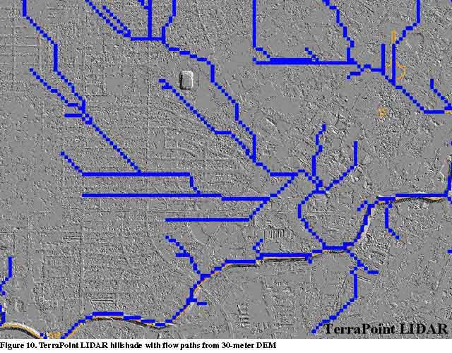
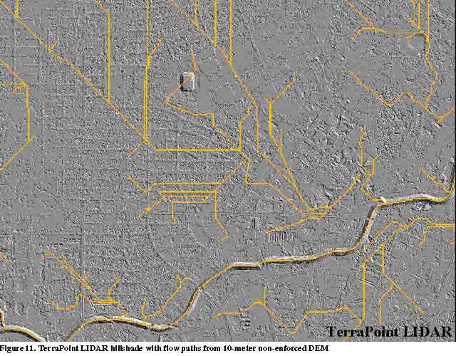
 An artificial flow path generated using the standard USGS 30-meter Level 2 DEM produced the results seen in Figure 10. Brays Bayou is adequately represented, but other portions of the drainage network appear random and do not reflect the actual landscape. Both 10-meter non-enforced and 10-meter drainage-enforced DEMs yield equally chaotic flow patterns in this urban area with few mapped surface drainage features (Figure 11).
The Use of LIDAR Data
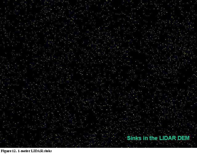
DEMs produced using LIDAR data offer a high-resolution alternative for surface modeling in low-relief areas. The prime benefit offered by LIDAR is its capability to capture small variations in relative surface relief with a vertical accuracy of 0.1-0.2 meter. Hydrologic modeling with LIDAR contains obstacles of its own. First, LIDAR data must be carefully filtered to eliminate reflectances from vegetation and other features unrelated to surface topography. In many instances, "bare-earth" LIDAR data retains far too much detail for current hydrologic modeling software to manage over areas of any substantial size. The extraordinary vertical accuracy of LIDAR technology means that LIDAR data contain enormous numbers of sinks. Figure 12 illustrates sinks present in the Houston study area in the 1-meter, bare-earth-filtered LIDAR data. These must be removed before further analysis can take place. Sink removal is an iterative procedure since removing one sink often creates one or more new sinks. With 1-meter resolution LIDAR data, the process can be self-destructive, and sometimes results in a contorted surface that no longer reflects terrain.
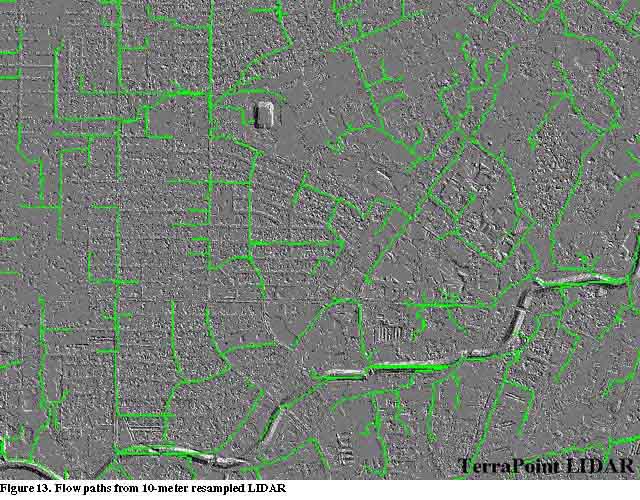
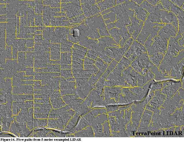
 One solution is to sub-sample the 1-meter, filtered LIDAR data. By starting with a 10-meter resampled version of the Bellaire LIDAR data, a much better representation of artificial flow paths was produced (Figure 13). The process was repeated using a 5-meter resampled version (Figure 14). It is obvious that the experiments using LIDAR-derived surface models result in better simulations of real drainage in an area where heavy runoff flows down streets and into storm drains.
Conclusions
Digital elevation models are available in a variety of horizontal and vertical resolutions. The 100-meter DTED1 data have been replaced by more accurate and useful 30-meter Level 2 DEMs available from the USGS. The 30-meter profile DEMs provide a generalized rendering of landforms appropriate only for regional studies at the scale of several thousand square kilometers. For hydrologic modeling, these surfaces perform poorly in areas of moderate topographic variation and not at all in flatter areas.
10-meter profile DEMs capture considerably more geomorphological detail and are appropriate for areal studies at 1:24,000 scale. Drainage enforcement improves the performance of 10-meter DEMs in many cases by more clearly delineating stream courses.
The surfaces of low-lying and extremely flat areas may not be adequately represented using DEMs created using hypsography data extracted from 1:24,000 scale USGS topographic maps. LIDAR technology offers a method to collect more accurate and detailed elevation data, but the datasets are large, need to be carefully filtered and may present problems for current software applications.
Acknowledgements
The authors wish to thank Jack Hill, Vice President of Environmental/Information Systems, of the Houston Advanced Research Center for graciously providing the TerraPoint LIDAR data used for this research.
Appendix
Spatial.DEMFill Avenue Code
' Title: Spatial.DEMFill
'
' Source: Arcview Spatial Analyst Sample Files
'
' Topics: Spatial Analyst, Hydrologic modeling
'
' Description: Takes a grid theme and fills all sinks, areas of
' internal drainage, contained within it. The aGrid.FlowDirection,
' aGrid.Sink, aGrid.Watershed, aGrid.ZonalFill, and aGrid.Con
' requests is used to fill the sinks. The process of filling
' sinks can create sinks, so a looping process is used until all
' sinks are filled. One cell sinks are not filled. Sinks of
' any depth are filled.
'
' Requires: The Spatial Analyst extension to be loaded. The script
' also requires an active view with an active grid theme that
' represents a surface. The grid theme should be the only active
' theme in the view.
'
' Self:
'
' Returns:
'

theView = av.GetActiveDoc

' fill active GTheme
theTheme = theView.GetActiveThemes.Get(0)

' fill sinks in Grid until they are gone
elevGrid = theTheme.GetGrid
sinkCount = 0
numSinks = 0
while (TRUE)
  flowDirGrid = elevGrid.FlowDirection(FALSE)
  sinkGrid = flowDirGrid.Sink
  if (sinkGrid.GetVTab = NIL) then
    ' check for errors
    if (sinkGrid.HasError) then return NIL end
    sinkGrid.BuildVAT
  end
  ' check for errors
  if (sinkGrid.HasError) then return NIL end
  if (sinkGrid.GetVTab <> NIL) then
    theVTab = sinkGrid.GetVTab
    numClass = theVTab.GetNumRecords
    newSinkCount = theVTab.ReturnValue(theVTab.FindField("Count"),0)
  else
    numClass = 0
    newSinkCount = 0
  end
  if (numClass < 1) then
    break
  elseif ((numSinks = numClass) and (sinkCount = newSinkCount)) then
    break
  end
  waterGrid = flowDirGrid.Watershed(sinkGrid)
  zonalFillGrid = waterGrid.ZonalFill(elevGrid)
  fillGrid = (elevGrid < (zonalFillGrid.IsNull.Con(0.AsGrid,zonalFillGrid))).Con(zonalFillGrid,elevGrid)
  elevGrid = fillGrid
  numSinks = numClass
  sinkCount = newSinkCount
end

' rename data set
aFN = av.GetProject.GetWorkDir.MakeTmp("fill", "")
elevGrid.Rename(aFN)

' create a theme
theGTheme = GTheme.Make(elevGrid)

' set name of theme
theGTheme.SetName("Filled"++theTheme.GetName)

' add theme to the view
theView.AddTheme(theGTheme)
Hydrologic Functions Avenue Example
'Name: Hydrologic_Functions
'Arthor: PR Blackwell
'             Forest Resoucres Institute
'Date:    July 11, 19999
'Description: Quick and dirty implementation of
'                     Spatial Analysit hydrologic modeling functions
'
'make sure we have a view up
theview = av.getActiveDoc
if (theView.is(View).NOT) then
  msgbox.error("Active Document must be a View","Exiting")
  exit
end

'get the grid to process
theThemes = theView.GetActiveThemes
theGrids = list.Make
for each t in theThemes
  if ( t.is(Grid) ) then
    theGrids.Add(t)
  end
end
if ( theThemes.Count <> 1 ) then
  elevGTheme = msgbox.list(theThemes,"Select the grid to process","Select Grid")
else
  elevGTheme = theThemes.get(0)
end
theName = elevGTheme.GetName
elevGrid = elevGTheme.GetGrid

' claculate flow direction
flowDir = elevGrid.FlowDirection(false)

'make a theme and add it to the view add it to the view
if (flowDir.hasError) then
  return nil
end
flowTheme = GTheme.Make(flowDir)
flowTheme.SetName(theName + ".fd")
theView.AddTheme(flowTheme)

' identify sinks
sink = elevGrid.sink
if (sink.hasError) then
  return nil
end
sinkTheme = Gtheme.Make(sink)
sinkTheme.SetName(theName + ".snk")
theView.AddTheme(sinkTheme)

'calcuate watershed
watershed = flowDir.Watershed(elevGrid)
if (watershed.hasError) then
  return nil
end
watershedTheme = GTheme.Make(watershed)
watershedTheme.SetName(theName + ".wsd")
theView.AddTheme(watershedTheme)

'calculate flow accumulation
flwAcc = flowDir.FlowAccumulation(nil)
if (flwAcc.hasError) then
  return nil
end
flwAccTheme = GTheme.Make(flwAcc)
flwAccTheme.SetName(theName + ".fa")
theView.AddTheme(flwAccTheme)