Design and Implementation of the Solar Analyst:
an ArcView Extension for Modeling Solar Radiation at Landscape
Scales
ABSTRACT
Incoming solar radiation (insolation) is the primary driving force for
Earth's physical, biological, and industrial systems. Knowledge of the
amount of insolation at various geographic locations is desirable for application
in such diverse fields as solar energy utilization, civil engineering,
agriculture, forestry, meteorology, environmental assessment, and ecological
research. For most geographical areas, however, insolation data are not
available. Simple interpolation and extrapolation of point-specific measurements
are typically not feasible, because insolation can vary significantly within
short distances due to topographic heterogeneity and nearground features.
While some geographical information systems (GIS) based solar radiation
modeling capabilities have been developed, there is a need for expanded
functionality, accuracy, and calculation speed. We developed the Solar
Analyst as an ArcView GIS extension, using C++, Avenue, and the GridIO
library. The Solar Analyst is a comprehensive geometric solar radiation
modeling tool. It calculates insolation maps using digital elevation models
(DEMs) for input. Highly optimized algorithms account for the influences
of the viewshed, surface orientation, elevation, and atmospheric conditions.
The Solar Analyst model was validated by comparing calculated temporal
and spatial patterns of insolation in the vicinity of Rocky Mountain Biological
Laboratory (RMBL) with detailed monitoring of insolation, weather, and
vegetation. The Solar Analyst provides a convenient and effective tool
for understanding spatial and temporal variation of insolation at landscape
and local scales.
Contents
1. Introduction: Spatial Solar Radiation Models
1.1 Importance of Understanding Landscape Patterns of Solar Radiation
Incoming solar radiation (insolation), with a continual input of 170 billion
megawatts to the earth, is the primary driver for our planet's physical
and biological processes (Geiger 1965, Gates 1980, Dubayah and Rich 1995,
1996). Almost all human activities (agriculture, forestry, building design,
and land management) ultimately depend upon insolation. At a global scale,
the latitudinal gradients of insolation, caused by the geometry of Earth's
rotation and revolution about the sun, are well known. At the landscape
scale, topography is the major factor modifying the distribution of insolation.
Variability in elevation, surface orientation (slope and aspect), and shadows
cast by topographic features create strong local gradients of insolation.
This leads to high spatial and temporal heterogeneity in local energy and
water balance, which determines microenvironmental factors such as air
and soil temperature regimes, evapotranspiration, snow melt patterns, soil
moisture, and light available for photosynthesis. These factors in turn
affect the spatial patterning of natural processes and human endeavor.
Accurate insolation maps at landscape scales are desired for many applications.
Although there are thousands of solar radiation monitoring locations throughout
the world (many associated with weather stations), for most geographical
areas accurate insolation data are not available. Simple interpolation
and extrapolation of point-specific measurements to areas are generally
not meaningful because most locations are affected by strong local variation.
Accurate maps of insolation would require a dense collection station network,
which is not feasible because of high cost. Spatial solar radiation models
provide a cost-efficient means for understanding the spatial and temporal
variation of insolation over landscape scales (Dubayah and Rich 1995, 1996).
Such models are best made available within a geographic information system
(GIS) platform, whereby insolation maps can be conveniently generated and
related to other digital map layers.
1.2 Spatial Solar Radiation Models
Spatial insolation models can be categorized into two types: point specific
and area based. Point-specific models compute insolation for a location
based upon the geometry of surface orientation and visible sky. The local
effect of topography is accounted for by empirical relations (Buffo et
al. 1972, Frank and Lee 1966, Kondrtyev 1969), by visual estimation (Swift
1976, Flint and Childs 1987), or, more accurately, by the aid of upward-looking
hemispherical (fisheye) photographs (Rich 1989, 1990, Rich et al. 1999).
Point-specific models can be highly accurate for a given location, but
it is not feasible to build a specific model for each location over a landscape.
In contrast, area-based models compute insolation for a geographical area,
calculating surface orientation and shadow effects from a digital elevation
model (DEM) (Hetrick et al. 1993a, 1993b, Dubayah and Rich 1995, 1996,
Rich et al. 1995, Kumar et al. 1997). These models provide important tools
for understanding landscape processes. The SolarFlux model (Hetrick et
al. 1993a, 1993b, Rich et al. 1995), developed for use within the ARC/INFO
GIS platform (Environmental Systems Research Institute [Esri], Redlands,
CA), simulates the influence of shadow patterns on direct insolation using
the ARC/INFO Hillshade function at discrete intervals through time. Solarflux
was implemented in the Arc Macro Language (AML), which strongly limits
its computation speed and its accessibility. Kumar et al. (1997) developed
a similar model using ARC/INFO and the GENAMAP GIS software (GENASIS, Australia).
Whereas point-specific models can be highly accurate for a specific location,
area-based models can calculate insolation for every location over a landscape.
A new generation of spatial models is needed that combines these respective
advantages, providing rapid and accurate maps of insolation over landscape
scales.
1.3 Features of the Solar Analyst
Herein we describe the design and implementation of the Solar Analyst,
a spatial solar radiation model implemented as an ArcView GIS (Esri) extension.
TopoView is a counterpart of the Solar Analyst implemented to run in the
Arc/Info GIS platform (Esri) rather than in ArcView. Except for some details
of the user interface, the following discussion applies to both the Solar
Analyst and TopoView. First we explain the underlying theory, design considerations,
and implementation of the Solar Analyst. Then, we validate the Solar Analyst
by comparing simulations with temporal and spatial analyses of empirical
data from the vicinity of Rocky Mountain Biological Laboratory (RMBL).
Finally, we explore the application of the Solar Analyst to examine landscape
patterns of insolation. The Solar Analyst draws from the strengths of both
point-specific and area-based models. In particular, the Solar Analyst
generates an upward-looking hemispherical viewshed, in essence producing
the equivalent of a hemispherical (fisheye) photograph (Rich 1989, 1990)
for every location on a DEM. The hemispherical viewsheds are used to calculate
the insolation for each location and produce an accurate insolation map.
The Solar Analyst can calculate insolation integrated for any time period.
It accounts for site latitude and elevation, surface orientation, shadows
cast by surrounding topography, daily and seasonal shifts in solar angle,
and atmospheric attenuation. The Solar Analyst has the following advantages
over previously developed models:
-
versatile outputs: creates maps of direct, diffuse, global radiation,
and direct radiation duration for any period (instantaneous, daily, monthly,
biweekly .); also calculates skyview factors, sunmaps and skymaps, viewsheds,
and horizon angles; analyses can be performed for whole DEMs, restricted
areas, or specific cells;
-
simple input: uses digital elevation models (DEMs) and a few readily
available parameters;
-
fast and accurate: uses an advanced viewshed algorithm for calculations;
-
easy to use & broad accessibility: based in ArcView, which supplies
the Solar Analyst with mapping, query, graphing, and statistical analysis
functions in a powerful desktop GIS platform.
2. Theory, Design, and Implementation
of the Solar Analyst
2.1 Theory: Use of Hemispherical Viewsheds in Solar Radiation Models
Hemispherical Viewshed Algorithm: Solar Radiation originating from
the sun travels through the atmosphere, is modified by topography and other
surface features, and then is intercepted as direct, diffuse, and reflected
insolation components. Generally, direct radiation is the largest component
of total radiation, and diffuse radiation is the second largest component.
Radiation reflected to a location from surrounding topographic features
generally accounts for a small proportion of total incident radiation and
for many purposes can be neglected (Gates 1980, Rich 1989, 1990, Hetrick
et al. 1993a, 1993b, Kumar 1997). Rich (1994) developed an algorithm for
rapid insolation calculation which, until now, has only been partially
implemented in point-specific models including Canopy (Rich 1989, 1990)
and Hemiview software (Rich et al. 1999) used for analysis of hemispherical
photography. This hemispherical viewshed algorithm serves as the core of
the Solar Analyst.
Viewshed Calculation: Viewsheds are calculated for each cell
of the input DEM. A viewshed is the angular distribution of sky obstruction.
This is similar to the view provided by upward-looking hemispherical (fisheye)
photographs. A viewshed is calculated by searching in a specified set of
directions around a location of interest (Fig. 1A), determining the maximum
angle of sky obstruction, also referred to as horizon angle, in each direction
(Fig. 1B)(Dozier and Frew 1990). For other unsearched directions, horizon
angles are calculated using interpolation (Fig. 1C). Then the horizon angles
are converted into a hemispherical coordinate system, in particular utilizing
an equiangular hemispherical projection, which represents a three-dimensional
hemisphere of directions as a two-dimensional grid (Fig. 1D). The resolution
of the viewshed grid must be sufficient to adeduately represent all sky
directions, but small enough to enable rapid calculations, e.g., 200 x
200 cells, 512 x 512 cells. Each grid cell is assigned a value that
corresponds with visible versus obstructed sky directions. The grid cell
location, row and column, corresponds to a zenith angle q
(angle relative to the zenith) and an azimuth angle a
(angle relative to north) on the hemisphere of directions.
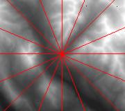
1A) Horizon angles are traced along a specified set of directions.
1B) Horizon angles are calculated for each direction.
1C) Horizon angles are interpolated for all directions.
1D) Horizon angles are converted to a hemispherical coordinate system.
1E) The resulting viewshed for a location represents which sky directions
are visible
and which are obscured. Numbers represent the calculated horizon angles.
Fig 1. Calculation of the viewshed for one cell of a DEM.
Sunmap Calculation: The amount of direct solar radiation originating
from each sky direction is represented by creating a sunmap in the same
hemispherical projection as for the viewshed (Fig. 2). The skymap
specifies suntracks, the apparent position of the sun as it varies through
time. In particular, suntracks are represented by discrete sky sectors,
defined by sun position at intervals through the day and season (e.g.,
half-hour intervals through the day and month intervals through the season).
The position of the sun (zenith and azimuth angles) is calculated based
on latitude, day of year, and time of day using standard astronomical formulae
(modified version of Gates 1980). Zenith and azimuth angles are projected
into two-dimensional grids with the same resolution used for viewsheds.
Two sunmaps are created, one to represent periods between the winter solstice
and the summer solstice (December 22 to June 22) and the other to
represent periods between the summer solstice and the winter solstice (June
22 to December 22). Each sky sector of the sunmap is flood-filled with
a unique identification number. For each sector, the time duration, the
azimuth and zenith at its centroid are calculated. This calculation also
accounts for partial sectors near the horizon.
Fig. 2. Annual sunmaps for 39o N latitude using 0.5 hour
intervals
through the day and month intervals through the year.
Penumbral Effects: For sunmaps that represent one day or less,
penumbral effects must be taken into account. The Solar Analyst uses a
solar disc semidiameter of 0.00466 radians near the zenith (0.2668o)
and larger values near the horizon (up to 1.6o) (U.S. Department
of Energy 1978) (Fig. 3). The solar disc appears larger near the horizon
due to refraction but it does not differ significantly from 0.5o
after the sun has risen above an elevation angle of approximately 10o.
Fig. 3. Penumbral effects are accounted for by constructing sunmaps
with consideration of the solar disc size.
Note that the sun track becomes wider near the horizon due to
refraction.
Skymap Calculation: Unlike direct insolation, which only originates
from directions along the suntrack, diffuse solar radiation can originate
from any sky direction. Skymaps are constructed by dividing the whole sky
into a series of sky sectors defined by zenith and azimuth divisions. Each
sector is flood-filled with a unique identification number (Fig. 4). The
zenith and azimuth angles of the centroid of each sector are calculated.
Sky sectors must be small enough that the centroid zenith and azimuth angles
reasonably represent the direction of the sky sector in subsequent calculations
(e.g., sky sectors representing 5.625o zenith intervals [16
zenith divisions] and 22.5o azimuth intervals [16 azimuth divisions]).
Fig. 4. A skymap with sky sectors defined by 16 zenith divisions and
16 azimuth divisions.
Overlay of Viewsheds with Sunmaps and Skymaps: The skymap and
sunmaps are overlaid on the viewshed (Figure 5). Gap fraction, the proportion
of unobstructed sky area in each skymap or sunmap sector, is calculated
by dividing the number of unobstructed cells by the total number of cells
in that sector.
Fig 5. Overlay of a viewshed on a sunmap (upper) and a skymap (lower).
Shaded areas are obstructed sky directions.
Direct Solar Radiation Calculation: For each sunmap sector that
is not completely obstructed, solar radiation is calculated based on gap
fraction, sun position, atmospheric attenuation and ground receiving surface
orientation. A simple transmission model (Rich 1989, 1990, Pearcy 1989,
Monteith and Unsworth 1990, Gates 1980, List 1971), which starts with the
solar constant and accounts for atmospheric effects based on transmittivity
and air mass depth, is implemented using the following equations.
Dirtot = SDir
q,a
(1)
Total direct insolation (Dirtot) for a ground location
is the sum of the direct insolation (Dir q,a)
from all sunmap sectors. The direct insolation from the sunmap sector with
a centroid at zenith angle q and azimuth
angle a is calculated using equation
2.
Dirq,a = SConst
*
tm(q)
* SunDurq,a * SunGapq,a
*
cos(AngIn q,a)
(2)
where:
SConst is the solar flux outside the atmosphere
at the mean earth-sun distance, know as solar constant. Estimates of the
solar constant range from 1338 to 1368 WM-2. As a result of
more precise measurements, the Commission for Instruments and Methods of
Observation in 1981 agreed to adopt the World Radiation Center (WRC) solar
constant (1367 WM-2), as is used in the Solar Analyst.
Solar constant fluctuates slightly, a few tenths of a percentage over periods
of years (Iqbal 1983), and this can be accounted for by differences in
the distance between the earth and sun from the mean earth-sun distance;
t is transmittivity of the
atmosphere (averaged over all wavelengths) for the shortest path (in the
direction of the zenith);
m(q) is the relative optical path
length (measured relative to the zenith path length). It is determined
by the solar zenith angle and elevation above sea level. For zenith angles
less than 80o, it can be calculated using equation 3, below.
For zenith angles greater than 80o refraction is important.
Various astronomical tables provide corrections for refraction at zenith
angles greater than 80o (e.g., List 1971, Table 137; Monteith
and Unsworth 1990, p. 40).
SunDurq,a is the
time duration represented by the sky sector. For most sectors, it is equal
to the day interval multiplied by the hour interval. For partial sectors
(near the horizon), the duration is calculated using spherical geometry;
SunGapq,a is the gap fraction
for the sunmap sector;
AngIn q,a is the angle
of incidence between the centroid of the sky sector and the axis normal
to the surface. It can be calculated using equation 4, below. The effect
of surface orientation is accounted for by multiplying by the cosine of
the angle of incidence.
m = EXP(-0. 000118 * Elev - 1. 638 * 10-9 * Elev2)
/cos(q)
(3)
where:
m is relative optical path length;
q is the solar zenith angle;
Elev is elevation above sea level in meters.
AngIn q,a = acos[Cos(q)*Cos(Gz)+Sin(q)*Sin(Gz)*Cos(a-Ga)]
(4)
where:
AngInSky q,a is
the angle of incidence between the intercepting surface and a given sky
sector with a centroid at zenith angle q
and azimuth angle a;
Gz is the surface zenith angle;
Ga is the surface azimuth angle.
Diffuse Solar Radiation Calculation: For diffuse radiation the uniform
diffuse model and the standard overcast diffuse model are typically implemented
(Rich 1989, 1990, Pearcy 1989) with satisfactory results. In a uniform
diffuse model, sometimes referred to as a "uniform overcast sky (UOC)",
incoming diffuse radiation is the same from all sky directions. In a standard
overcast (SOC) diffuse model, diffuse radiation flux varies with zenith
angle. Both these models are implemented in the Solar Analyst. Other models
can readily be implemented in the future, including anisotropic models.
For each sky sector the diffuse radiation at its centroid is calculated,
integrated over the time interval, and corrected by the gap fraction and
angle of incidence using equation 5.
Difq,a = Rglb
* Pdif * Dur * SkyGapq,a
* Weight q,a * cos(AngIn
q,a)
(5)
where:
Rglb is the global normal radiation (see
equation 6 below);
Pdif is the proportion of global normal radiation
flux that is diffuse. Typically it is approximately 0.2 for clear sky conditions
and ranges from 0. 6 to 0. 7 for very cloudy sky conditions;
Dur is the time interval for analysis;
SkyGapq,a is the gap fraction
(proportion of visible sky) for the sky sector;
Weight q,a is proportion
of diffuse radiation originating in a given sky sector relative to all
sectors (see equation 7, below);
AngIn q,a is the
angle of incidence between the centroid of the sky sector and the intercepting
surface.
Rglb can be calculated by summing the direct radiation
from every sector (including obstructed sector) without correction for
angle of incidence, and then correcting for proportion of direct radiation,
which equals to 1- Pdif.
Rglb = (SConst
S (tm(q)
)
)/ (1 - Pdif)
(6)
For the uniform sky diffuse model, Weight q,a
is calculated as follows:
Weight q,a = (cosq2
- cosq1) / Divazi
(7)
where:
q1and
q2
are the bounding zenith angles of the sky sector;
Divazi is the number of azimuthal divisions in the
skymap.
For the standard overcast sky model, Weight
q,a is calculated as follows:
Weightq,a = (2cosq2
+ cos2q2 - 2cosq1
- cos2q1) / 4 * Divazi
(8)
Total diffuse solar radiation for the location (Diftot)
is calculated as the sum of the diffuse solar radiation (Dif
q,a) from all the skymap sectors:
Diftot = SDif
q,a
(9)
2.1.4 Global Solar Radiation Calculation
Global radiation (Globaltot) is calculated as the
sum of direct and diffuse radiation of all sectors. The above processes
are repeated for each location on the topographic surface, thus producing
an insolation map for the whole study area.
Globaltot = Dirtot + Diftot
(10)
2.2 Design and Implementation of the Solar Analyst
Overall Design: The hemispherical viewshed algorithm and associated
calculations were implemented in C++ library format, which can be flexibly
loaded in other software in both PC and UNIX platforms. For PC use the
program was compiled in Dynamic Link Library (DLL) format (solarlib.dll).
There are three C++ classes in the calculation engine:
The solar class controls the main loop of the entire model.
It reads the input DEM and calculates the horizon angles for each pixel
in a DEM. Then it passes the horizon angles to the other two classes for
the calculation of insolation. Finally, it gets the results and saves the
results in files.
The sun class calculates local solar time, sun declination, sun
position, sun rise/set time, day length, and solar constant. Also it calculates
the day of year from solar declination values.
The sky class creates skymaps and sunmaps, converts horizon angles
to viewsheds, overlays the skymaps and sunmaps with viewshed, and computes
gap fraction and solar radiation for each sector.
The program is highly optimized and uses fast algorithms for computations,
in particular, a fast line algorithm for searching maximum horizon angle,
fast calculation of horizon angle, fast flood-fill function to assign identifications
(visible versus obstructed) to sky regions in the viewshed, and fast overlay
of the viewshed with sunmaps and skymaps. Also, the program creatively
implemented calculations of partial sector information, penumbral effects,
and dual sunmaps when needed to account for overlapping sunpaths for any
period of time. To speed the calculation, instead of frequent access to
a physical disk drive, calculations are performed mainly in the RAM. For
example, the DEM is read into RAM when it is first opened and then used
extensively for all subsequent viewshed calculations. The sunmaps and skymaps
are created and stored in RAM, so they can be rapidly overlaid on viewsheds.
The program has been extensively tested to assure its quality and stability.
Data input and output were implemented using the ArcView GridIO library
(Fig 6), which comes with the ArcView Spatial Analyst. The user interface
(Fig 7), which permits parameter input and calls the calculation engine,
was developed using the ArcView Dialog Designer and Avenue. Because Avenue
can not directly call C++ class member functions, another DLL, which calls
the C++ member functions using nonmember functions, was developed as the
interface between the calculation engine and Avenue. The Solar Analyst
is based in ArcView, which supplies the Solar Analyst with its mapping,
query, graphing and statistic analysis functions.
Fig. 6. Flow diagram showing the design of the Solar Analyst.
7A) Buttons and other tools allow calculation for interactively selected
locations.
7B) Menus provide access to full capabilities.
7C) The output dialog window permits specification of custom output.
7D) The topographic parameter window permits specification of calculation
parameters
relevant to the topographic surface being analyzed.
7E) The sky parameter window permits specification of parameters
relevant to sunmap and skymap calculations.
Fig 7. User interface of the Solar Analyst.
Program Specifications: While the model algorithm appears somewhat
complex, the Solar Analyst is designed to be easy to use. The Solar Analyst
only requires a few input parameters and users do not need to have extensive
knowledge of atmospheric physics or meteorology.
Output of the Solar Analyst includes the following:
-
Direct insolation, diffuse insolation, global insolation,
direct
radiation duration, and skyview factor in Arc/Info Grid format
or ASCII text format;
-
Skymaps and sunmaps in Arc/Info Grid format;
-
Viewsheds (for specific cells) in Arc/Info Grid format;
-
Horizon angles in ASCII text format.
Input parameters to the Solar Analyst include the following:
-
DEM file name: specifies an Arc/Info Grid file location. User has
options to choose the following analysis areas:
-
Whole DEM.
-
Area covered by a mask grid (in Arc/info Grid format). For pixels
near the edges of a DEM, the viewshed calculated may not be true because
of the edge problems. Better results can be obtained if viewsheds are calculated
only for areas away from the edge. This mask function is implemented for
such purposes. While the Solar Analyst only calculates viewsheds for the
masked area, it can use cells out of the mask grid boundary in calculating
horizon angles.
-
Locations by rows and columns in ASCII format.
-
Locations by x and y coordinates in ASCII format.
-
Locations from a point coverage in Arc/Info coverage or shape file
format,
-
Locations of graphic points in the view. This allows the user to
specify points interactively and calculate the insolation or viewshed.
-
Object height offset: this is used for location calculation only.
For example, weather station sensors and solar powered devices are usually
mounted above the ground.
-
Slope and aspect information: users can choose from the following
options:
-
Grids: as calculated from DEMs, or in some special cases provided
by the user for a unique purpose.
-
Constant values: these values can be different from slope and aspect
values calculated from the DEM. For example, solar radiation sensors are
usually flat and mounted horizontally.
-
ASCII files: field surveys often measure slope and aspect for each
sample location. These measured values are generally more accurate than
DEM derived values. Using measured values can improve the accuracy of analysis.
-
None: perform calculations so that radiation values are corrected
for angle of incidence. For example, some solar powered devices automatically
change orientation to track the sun. In another example, a plant may have
leaves in all orientations (random hemispherical distribution of orientations).
-
Directions for viewshed calculation: because the viewshed calculation
is highly intensive, horizon angles are only traced in the number of directions
specified and horizon angles for other directions are calculated by interpolation.
-
Elevation unit: in correction for air mass optical depth, the Solar
Analyst performs calculations using elevation in meters. However, if the
input DEM is in units other than meters, the program will convert the elevation
into meters for calculations.
Sun/sky input parameters of the Solar Analyst include the following:
-
Site latitude: this is used in such calculations as solar declination
and solar position. Because the Solar Analyst is designed for landscape
scales and local scales, it is acceptable to use one latitude value for
the whole DEM.
-
Sky size: this is the resolution for the viewshed, skymap, and sunmap.
-
Zenith and azimuth divisions: these define the sky sectors of the
skymap.
-
Diffuse radiation model: currently users can choose either the uniform
diffuse model or the standard overcast diffuse model.
-
Diffuse proportion: the proportion of global normal radiation flux
that is diffuse.
-
Transmittivity: because the program will correct elevation effects,
transmittivity should always be given for sea level. Also it is important
to note the inverse relation between transmittivity and diffuse proportion
when deciding values to use for calculations.
-
Time configuration: the time for which insolation is to be calculated
can be specified as follows:
-
Within one day: user can specify the day of year, starting time,
and ending time. When starting time equals the ending time, instantaneous
solar radiation is calculated.
-
Special days: for summer solstice, equinox, and winter solstice.
-
Multi-day: users can specify the start day, end day, year, day interval,
and hour interval for calculations. When end day is smaller than start
day, the end day is considered to be in the following year of the start
day. A day interval of 7 corresponds with weekly intervals, whereas a day
interval of 14corresponds with biweekly intervals.
-
Whole year with monthly intervals: this is a special multi-day calculation
in that the day intervals are not constant.
-
For each interval: this check box gives users the flexibility to
calculate total insolation or insolation for each session. For example,
for multiple days with a day interval of 7, checking this box will create
weekly insolation; otherwise, only the total insolation during the start
day and end day are calculated. In another example, for within day with
an hour interval of 1, checking this box will create hourly insolation
calculations; otherwise, only the total insolation over the day is calculated.
3. Methods
3.1 Study Site
We have been applying the Solar Analyst in our research concerning microclimate
and vegetation patterns in the vicinity of the Rocky Mountain Biological
Lab (RMBL), Colorado. Dramatic topographic variation, with elevations ranging
from 2532 m to 4340 m, leads to a diversity of vegetation communities (Langenheim
1962).
3.2 Weather Stations & Insolation Monitoring
Four weather stations have been established in the vicinity of RMBL (Fig.
8). One weather station (called the "research meadow" station) was
established in 1989 by the Environmental Protection Agency. The other three
(called the "upper meadow", "middle meadow", and "lower meadow" stations)
were established in June 1997 for research concerning climate change and
include monitoring of global insolation using Li-Cor pyranometers mounted
horizontally about 2 m above the ground (John Harte unpublished). Readings
were averaged and recorded using a Campbell data logger at hourly intervals
during summer of 1997 and at two-hour intervals thereafter.
3.3 Digital Elevation Model
We constructed a DEM for the vicinity of RMBL using 30-m resolution DEMs
for nine U.S. Geological Service 7.5' quadrangles: Gothic, Snowmass Mt.,
Maroon Bells, Hayden Peak, Oh-Be-Joyful, Pearl Pass, Axtell, Cement Mt.,
and Crested Butte. The RMBL vicinity DEM was used to calculate viewshed
and insolation. Locations of the weather stations were surveyed using
a differentially corrected Global Positioning System (Trimble Pathfinder).
Both the RMBL vicinity DEM and the weather station locations were converted
into a Universal Transverse Mercator projection (Fig. 8).
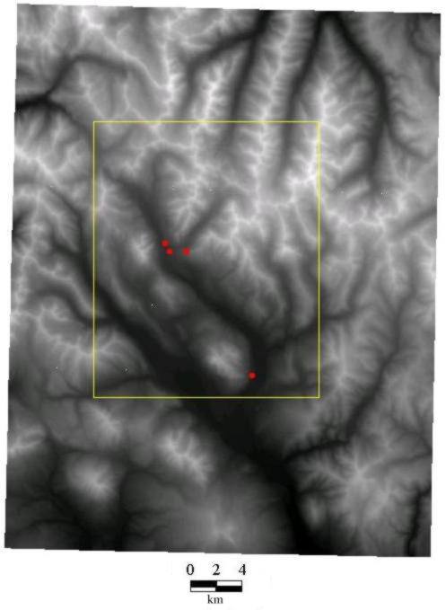
Fig. 8. RMBL vicinity DEM, weather station locations (red) and
calculation mask (yellow).
3.4 Viewshed Calculation and Hemispherical Photographs
Viewsheds were calculated for each location within the calculation mask
(fig 8). We compared the calculated and observed viewsheds for each weather
station using hemispherical photographs taken near the insolation sensor.
For viewshed calculations a 2m offset was added to account for the height
of the sensor and horizon angles were calculated at 64 directions.
3.5 Insolation Patterns
Temporal Patterns through the Day: Insolation on a typical
clear day, July 4, 1997, was calculated and compared with sensor values
for the "middle meadow" site. The sensor measurements were converted to
true local solar time using the equation for time to account for the time
zone meridian. Calculations used a transmittivity value of 0. 6 and a diffuse
proportion of 0. 2. Slope was set to zero, corresponding to the horizontal
surface of the insolation sensor. The viewshed was calculated along 64
directions to obtain good accuracy; sky size was set at 512 x 512 cells;
the skymap was created using 18 zenith divisions and 16 azimuth divisions;
and the sunmap was created using a 6-minute (0.1 hour) interval through
the day.
Annual Insolation Patterns: Monthly insolation was calculated
throughout the course of the year for the "research meadow" site assuming
transmittivity of 0.5 and diffuse proportion of 0.3. Again slope and aspect
were set to zero, the viewshed was calculated along 64 directions, sky
size was set at 512 x 512 cells, and the skymap was created using 18 zenith
divisions and 16 azimuth divisions. The sunmap was created using half-hour
intervals through the day and monthly intervals through the year.
Spatial Patterns of Insolation: The Solar Analyst was used to
calculate monthly direct, diffuse, global, and direct duration maps from
the RMBL DEM (4 maps x 12 months = 48 maps total). The program was run
on a Compaq Armada 7800 (333MHz CPU and 128M RAM). Parameters were set
to transmittivity of 0. 5, diffuse proportion of: 0. 3, 32 viewshed calculation
directions, a sky size of 200 x 200, a skymap of 8 zenith divisions and
8 azimuth divisions, and a sunmap of half-hour intervals through the day
and monthly intervals through the year. The DEM consists of 1,591,590 (1410
x 1113) grid cells. To avoid edge effects, insolation was only calculated
for the center area by applying a mask of 703 x 574 (403,522) cells (Fig.
8). When calculating viewshed, the pixels out of the mask were still used
to calculate horizon angles.
3.6 Inferring Insolation from Incomplete Data
A variety of appoaches have been employed when insolation data are incomplete
or unavailable. Based on our temporal and spatial analyses we examine the
validity of various of these approaches:
-
Using measurements from nearby monitoring stations to infer insolation
for a broader area: A histogram was constructed to permit examination
of the extent of spatial variation in annual global insolation, based on
the direct and diffuse maps of insolation for the study area.
-
Grouping aspect and slope: Summary statistics of insolation for
the month of June (minimum, maximum, and mean) were calculated for six
categories of slope and aspect in the study area: aspects of north vs.
south and slopes of 0-29o, 30-59o, and 60-90o.
These statistics permit examination of the validity of using such categories.
-
Using sinusoidal curves to simulate daily insolation patterns: Daily
insolation curves were calculated for four locations with different aspects
(north-, south-, east-, and west-facing) to examine the influence of orientation
on the shape of the daily insolation curve.
-
Calculating diffuse solar radiation as a proportion of direct or global
solar radiation: The same daily insolation curves for locations with
different aspects, along with their viewsheds, were used to examine the
validity of calculating diffuse radiation as a proportion of direct or
global measurments from sensors.
-
Using direct duration to estimate direct insolation: We calculated
correlation coefficient between direct duration and direct, diffuse, and
global radiation for each month based on the insolation maps for the study
area.
3.7 Sensitivity Analysis
A series of sensitivity analyses were used to assess the effects of different
input parameters on the outputs from from the Solar Analyst:
-
Viewshed Calculation Directions: To assess tradeoffs between calculation
speed and accuracy, we tested the sensitivity of the Solar Analyst to different
numbers of calculation directions using the RMBL DEM (a topographically
complex area) and another DEM in Kansas (a low-relief area). For each of
the two DEMs, horizon angles for three locations were computed at 8, 16,
24, 32, 40, 64, 128 and 360 directions. Calculated viewsheds were compared
with the 360-direction viewshed.
-
Sky resolution and skymap divisions: To assess tradeoffs between
calculation speed and accuracy, we tested the sensitivity of the Solar
Analyst to two sets of sky resolution and skymap divisions: 400 x
400 sky size with 16 x 16 skymap divisions and 200 x 200 size with 8 x
8 skymap divisions.
-
Sunmap divisions: To assess tradeoff between calculation speed and
accuracy, we tested the sensitivy of the Solar Analyst to various combinations
of sunmap divisions, ranging from 0.2 to 1.0 hour intervals through the
day and between one day and one month intervals through the year.
-
Elevation effects: We assessed the importance of elevation corrections
in the Solar Analyst by examining relations between elevation, optical
air mass, and insolation.
4. Results and Discussion
4.1 Viewsheds
The calculated and observed viewsheds match well (Fig. 9). The strongest
correspondence between calculated and observed viewsheds are for more distant
features, such as Gothic Mountain to the west and Whiterock Mountain to
the northeast. Small discrepencies exist toward the north and east
because of trees. In some cases such discrepencies can be more pronounced
either due to strong effects of nearby features such as trees or errors
inherent in a DEM.
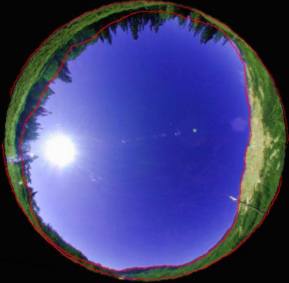
Fig. 9 Comparison of calculated viewshed with a hemispherical photo
4.2 Insolation Patterns
Temporal Patterns through the Day: There is excellent agreement
between the measured and calculated global insolation values through the
day (Fig. 10). Total insolation for the "middle meadow" site on July 4,
1997 was observed to be 8115. 4 w/m-2, of which direct was 6967.2
w/m-2 (85.9%) and diffuse was 1148.3 w/m-2 (14.1%).
Note that that insolation values jump at about 6:15 and drop around 17:20.
This results from the geometry of the viewshed, as can clearly be seen
by referring back to Fig. 8. The geometry of sky obstruction allows us
to predict when direct radiation drops off. Before 6:15 sky obstruction
by Whiterock Mountain blocked direct radiation and only the diffuse radiation
component contributed to global radiation. At about 17:20 the sun was blocked
by Gothic Mountain and the global insolation was again reduced to only
the diffuse radiation component.
Fig. 9 Comparison of calculated and observed insolation for typical
clear day
Annual Insolation Patterns: The annual pattern of monthly insolation
for the "research meadow" site diplays a distinct sinusoidal pattern, with
a peak near the summer solstice and a trough near the winter solstice (Fig.
11). This pattern is driven primarily by the shifting angle of the suntrack
with respect to the horizontal surface of interception. In the field
considerable variation exists from one day to another and from one year
to another, caused mainly by variation in cloud cover. The Solar Analyst
is able to calculate insolation for different atmospheric conditions, but
information about variation in transmittivity and diffuse proportion parameters
are not typically available. The Solar Analyst can only be used to examine
short-term non-systematic variation in cases where detailed insolation
monitoring is available for the region of interest. More commonly, the
Solar Analyst is best suited for comparing daily patterns and seasonal
patterns as they vary spatially.
Fig. 10 Annual pattern of direct, diffuse and global insolation for
average clear day for the weather station at the research meadow
Spatial Patterns of Insolation: It required three hours to calculate
the monthly direct, diffuse, global, and direct duration maps (48 maps
total). Maps of direct and diffuse insolation for the whole year are shown
in Figs. 11 and 12. Among the distinct patterns that can be observed by
inspection of the annual direct radiation map (Fig. 11) are distinctly
lower insolation on north-facing slopes as compared with south-facing slopes,
as well as lower insolation levels in landscape positions with high sky
obstruction along the suntrack (i.e., mountains toward the south, east,
or west). By contrast, variation in the annual diffuse insolation map results
primarily as a function of slope (higher slope causing lower values) and
sky obstruction in any direction (more sky obstruction causing lower values).
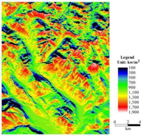
Fig 11. Map of annual direct insolation (note map quality reduced because
of file compression)
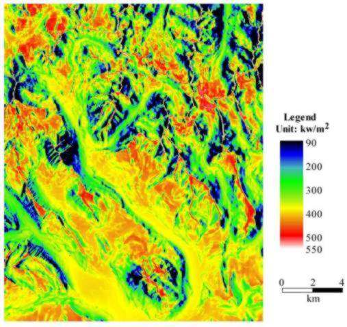
Fig 12. Map of annual diffuse insolation (note map quality reduced
because of file compression)
4.3 Inferring Insolation from Incomplete Data
Using measurements from nearby monitoring stations to infer insolation
for a broader area: Commonly studies use measurements at one weather
station to infer patterns for the its entire study area. This approach
can neglect the temporal and spatial variation of insolation. Iin many
situations, especially for mountainous regions, this approach is not effective.
Tremendous variation exists in insolation received at different spatial
locations (Fig. 13). In this example, the variation results directly from
variation in topography. Additional variation in insolation can result
because of spatial variation in atmospheric conditions, in particular cloud
cover.
Fig 13. Variation of annual insolation (KWH/m2) over
the study area.
Grouping aspect and slope: Commonly locations with similar slopes
and aspects are grouped in analysis to infer variation of insolation in
the landscape. In the northern hemisphere it is generally assumed that
south-facing slopes receive more insolation than north facing slopes, while
the converse is is assumed in the southern hemisphere. While south-facing
slopes do have mean insolation values higher than north-facing slopes during
the month of June (Table 1), the statistic demonstrate that there are many
cases where north-facing slopes receive more insolation than south-facing
slopes. This results because of local sky obstruction and the importance
of early and late times during the day when the suntrack is far to the
north.
Table 1. Summary statistics, according to aspect and slope category,
for insolation values in June (KWH/m2).
|
Aspect
|
Slope
|
Min
|
Max
|
Mean
|
|
North
|
0-29o
|
146
|
257
|
218
|
|
30-59o
|
90
|
253
|
183
|
|
60-90o
|
95
|
108
|
101
|
|
South
|
0-29o
|
138
|
261
|
219
|
|
30-59o
|
90
|
263
|
192
|
|
60-90o
|
99
|
167
|
141
|
Using sinusoidal curves to simulate daily insolation patterns: Symmetrical
sinusoidal curves have been widely used to simulate daily insolation patterns.
Symmetrical daily patterns generally only can occur for flat surfaces or
aspect directly north or south, and with symmetrical east-west sky obstruction.
Assymetrical daily insolation results from slope orientation to the east
or west and from assymetrical sky obstruction (Fig. 14). Further assymetry
of daily insolation patterns can result from variation in atmospheric conditions,
for example in locations where afternoon clouds are common.
Fig 14. Daily Insolation patterns for locations on different slopes.
Calculating diffuse solar radiation form direct or global solar radiation:
Various relations between diffuse and global or direct model has been formulated
(Liu and Jordan 1960, Erbs 1980). These models are used to calculate diffuse
radiation components when only global radiation striking a horizontal sensor
is measured, or when only direct insolation is calculated. These
models assume relations between diffuse and global or direct radiation
without considering differences in viewsheds. Further, these models
have been widely used, even in mountainous regions, to derive daily or
seasonal insolation patterns. A western slope may have as much as 100%
diffuse radiation in the morning while only 15% diffuse radiation in the
afternoon (Fig. XX). Similarly, some slopes may have 100% diffuse radiation
during the entire winter season, but with a low proportion of diffuse radiation
in the summer. High variability in slope orientation and viewsheds mean
that this approach is generally not valid.
Using direct duration to estimate direct insolation: In the absence
of solar radiation measurements, it is common practice to use direct duration
as an estimate of direct insolation. Correlations between duration
and direct measurements ares higher in winter than in summer; while correlations
between duration and diffuse measurements are higher in summer than in
winter (Table 2). Correlations between duration and global measurements
are higher in winter than in summer, but correlations can be as low as
0.41. The primary problem of using direct duration to predict insolation
is that it does not account for either the angle of incidence or the length
of the atmosphere traversed, both of which vary markedly through the day.
Table 2. Correlation between direct duration and radiation
|
Duration & Global
|
Duration & Direct
|
Duration & Diffuse
|
|
Jan.
|
0.7153
|
0.6922
|
0.3740
|
|
Feb
|
0.6642
|
0.6281
|
0.4714
|
|
Mar
|
0.5287
|
0.4567
|
0.6305
|
|
Apr
|
0.4128
|
0.2947
|
0.6929
|
|
May
|
0.4337
|
0.2954
|
0.6743
|
|
Jun
|
0.4576
|
0.3290
|
0.6640
|
|
Jul
|
0.4273
|
0.2927
|
0.6672
|
|
Aug
|
0.4226
|
0.2916
|
0.6914
|
|
Sep
|
0.4881
|
0.3995
|
0.6684
|
|
Oct
|
0.6386
|
0.5925
|
0.5200
|
|
Nov
|
0.7159
|
0.6907
|
0.3880
|
|
Dec
|
0.7352
|
0.7175
|
0.3343
|
4.4 Sensitivity Analysis
Viewshed Calculation Directions: A set of 32 calculation directions
were sufficient to obtain a mean error less than 0.5 degree for the complex
mountain topography around RMBL. By contrast, only 8 or 16 directions were
needed to obtain a mean error less than 0.5 degree for the gentle topography
in Kansas. are needed for such complex mountain
topography as RMBL. Because horizon angle calculation is computationally
intensive, users should select the minium set of azimuth directions that
suit their needs. Horizon angles at other directions are calculated using
simple linear interpolation.
Sky resolution: Similar results were obtained using 400 x 400
and 200 x 200 sky resolution. are highly similar. The correlation between
the calculated global insolation is 0. 99994 at winter and 0.99995 at summer.
The average value differs by less than 1%. Based on this testing, we concluded
that a 200 x 200 sky size is sufficient for most purposes. Increasing sky
size beyond this does not significantly improve model accuracy, but greatly
increases computation time. For example, doubling the sky resolution from
200 x 200 to 400 x 400 quadruples the computation time. The Solar Analyst
is implemented such that sky resolution is user defined. Further research
may reveal cases where higher sky resolutions may be required.
Skymap divisions: Increased number of skymap divisions does not
affect computation time greatly and does not improve global radiation much
as shown in the above test. The results because diffuse radiation is generally
a relatively small proportion of global radiation, and because we are using
uniform sky or standard overcast models. In most situations 8 x 8 sky divisions
is sufficient. In cases where diffuse radiation is of major interest, skymap
divisions should be increased to 16 x 16 or even more. Skymaps of 18 zenith
divisions (5-degree intervals) and 16 azimuth divisions (22.5-degree intervals)
are commonly employed for detailed studies (Rich et al. 1999).
Sunmap divisions: Changing sunmap divisions does not change computational
time much, but can improve calculation accuracy. In general, a 0.2 hour
interval through the day is sufficient for daily insolation calculations,
and a 0.5 hour interval is sufficient for multi-day calculations. The appropriate
interval through the year is usually determined based on user needs.
For example, it should be 7 for weekly calculations, 14 for biweekly calculations,
and monthly for monthly calculations.
Elevation effects: Generally, higher elevations receive more
insolation than lower elevations. This results both because higher elevation
have more open viewsheds and because the solar beam travels through less
air mass (Fig. 15). For the vicinity of RMBL, the air mass is approximately
half at the upper most elevation ( 4,340 m) as compared with the lowermost
elevation (2,532 m). While a change of 10 m has trivial effects on
air mass and insolation, a change from sea level to 5,000 m can result
in an increase of 52% in global radiation (Table 2). Another effect that
partially counterbalances less air mass at higher elevations involves increased
cloudiness with increasing elevation.
Fig 15. The relationship between elevation and zenith air mass
optical depth.
Table 3. Effects of elevation on insolation
|
Elevation (m)
|
Relative air optical depth at zenith
|
Insolation (w/m2) at average clear day
Flat and open surface at latitude 38.95N, 12:00pm at equinox
|
|
Direct
|
Diffuse
|
Global
|
|
0
|
1
|
435.9
|
120.2
|
556.1
|
|
10
|
0.999
|
436.3
|
120.4
|
556.7
|
|
1000
|
0.89
|
482.0
|
132.9
|
614.9
|
|
2000
|
0.78
|
528.1
|
145.7
|
673.8
|
|
3000
|
0.69
|
573.8
|
158.3
|
732.1
|
|
4000
|
0.60
|
618.4
|
170.6
|
789.0
|
|
5000
|
0.53
|
661.4
|
182.4
|
843.9
|
4.5 DEM Issues
DEM Quality: DEMs are used to derive three kinds of information:
elevation, slope and aspect, and viewsheds. Their effects on model accuracy
can be assessed in separately:
-
Elevation: Elevation is used directly in calculation of air optical
depth. Though, elevation can deviate significantly from actual values,
a 10 to 30 m error will only affect the air optical depth at 0.1%. Thus
elevation errors do not produce significant effects on model accuracy.
-
Slope and aspect: Poor DEM quality, limitations due to resolution,
and edge effects can lead to inaccurate slopes and aspects. This is a potentially
serious source of error because insolation values are corrected for angle
of incidence, which ultimately depends on surface slope and aspect. The
Solar Analyst has the ability to use surveyed slopes and aspects, which
can improve accuracy for various applications.
-
Viewsheds: Based on our experience, DEM does not generally change
viewsheds greatly, however further work is needed to assess cases where
viewshed errors may be significant.
One important index of DEM quality is its cell size. As grid cell increases,
topographic generalization occurs. While the average regional radiation
may not change much, values for some individual cells may change significantly.
The quality of DEMs, including the cell size, should be evaluated against
user needs. The commonly available 30 m USGS DEM is sufficient for most
environmental and ecological applications at landscape scales. Applications
that require high accuracy for specific locations may require higher resolution
DEMs.
DEM Projection Considerations: For viewshed calculations, the
Solar Analyst assumes DEMs are in a projection that preserves direction.
Most DEMs are available in projections that do not exactly preserve direction.
For some commonly used projections (e.g. UTM), slight rotation of the study
area to register correctly with true north can be sufficient to improve
accuracy.
4.6 Limitations
Clouds: The Solar Analyst does not currently model clouds, per se,
although clouds can be taken into account when estimating transmittivity
and diffuse proportion. Clouds are extremely hard to model or predict,
and detailed information, such as clouds distribution, thickness, cloud
type, are not available for most areas. If such data are available, the
Solar Analyst could readily be customized by adding a cloud skymap that
can be overlaid with the viewshed, skymap, and sunmap. Alternatively
cloud information could be included in specification of sector-specific
insolation when construction skymaps and sunmaps. For many purposes, in
particular involving multi-day insolation calculation, cloud effects can
be included by using an appropriate transmittivity and diffuse proportion.
Reflected Radiation: The Solar Analyst currently neglects the
contribution of reflected radiation from the ground. This is valid for
most uses. Reflected radiation is important for places where ground surfaces
have high albedo, for example, snow-covered surfaces. Reflected radiation
is complex because it varies with surface cover properties, surface orientation,
and sun position. However, the algorithm utilized in the Solar Analyst
permits calculation of simplified estimations of reflected radiation (Rich
1994). In the viewshed, direct and diffuse radiation come from visible
sky directions, while ground-reflected radiation comes from obstructed
directions. We can assign obstructed sky sectors a reflectance index that
estimates the reflectance from ground features. The reflected radiation
can then be calculated by summing the reflected radiation from obstructed
sectors in a manner similar to the way direct and diffuse radiation calculated.
Locations open to lower surfaces can receive reflected radiation from lower
elevations. In these cases a hemispherical view downward could be used
to account for upwelling radiation. In general,implement this approach
is challenging.
Ground Features: Generally, a DEM only describes the topographic
terrain and does not represent ground features such as plant canopies and
human structures. Such ground features can have a, which can affect ground
insolation strongly. If these ground features can be included in DEMs the
Solar Analyst can still be used. For example, in urban areas it is possible
to construct a high-resolution DEM that including buildings and other structures.
Irregular features, such as plant canopies can also be converted into DEMs,
but obtaining such data can be challenging (Rich et al. 1993, Price et
al. 1995). For detailed characterization of specific locations, hemispherical
photography can be a more appropriate technique (Rich 1989, 1990, Rich
et al. 1999). With minor modification, the calculation engine of the Solar
Analyst can use hemispherical photography to examine solar radiation regimes
for specific locations. Further work is needed to fully integrate the Solar
Analyst with spatially explicit canopy models such as those of Fournier
et al. (1997).
4. CONCLUSION
In the development of the Solar Analyst, we implemented a fast and effective
algorithm that permits accurate calculation of topographic influences on
solar radiation over local and landscape scales. Considerable insolation
variation exists between different landscape positions. Such variations
have a significant effect on the ground energy balance, water balance,
and nutrient cycles, which directly or indirectly affect natural processes
and human activities. As an example of its application, we are using the
Solar Analyst and meteorologic measurements in models of spatial patterns
of microclimate factors, including air temperature, soil temperature, and
soil moisture. This topoclimatic modeling approach can lead us to a better
understanding of the relationship between microclimate and vegetation distribution
patterns, as well as potential habitat shifts under climate change scenarios.
Preliminary analyses demonstrate that commonly used techniques (generalization
from nearby insolation monitoring, prediction by slope and aspect categories,
estimating direct radiation from direct duration, etc.) are not sufficiently
accurate for generalization of insolation patterns to a landscape scales.
The Solar Analyst serves as a powerful tool for analyzing spatial and temporal
patterns of insolation at local and landscape scales. Applications span
a broad range of fields, including forestry, agriculture, hydrology, micrometerology,
environmental assessment, and ecological research. The Solar Analyst also
promises to be useful in engineering and design fields, for such applications
such as site assessment, building design, solar collector design, and topographic
radiometric correction for remote sensing.
Acknowledgements
This research was supported by the Information Telecommunication and Technology
Center (ITTC), the Kansas Biological Survey, the University of Kansas General
Research Fund, and Helios Environmental Modeling Institute. We would like
to give thanks to Susannah Geer for providing editorial comments and field
assistance and to Brett Greene for providing field assistance. We also
thank John Harte, Jennifer Dunne, and Marc Fischer at the University of
California, Berkeley, who provided weather and other environmental data,
gathered with support from National Science Foundation grants DEB-96-2889
and DEB-96-23258 to John Harte.
References
Buffo, J., L.J. Fritschen, and J.L. Murphy. 1972. Direct solar radiation
on various slopes from 0o to 60o north latitude.
U.
S. Forest Service Pacific Northwest Forest Range Experimental Station Research
Paper, PNW-142.
Dozier, J. and J. Frew. 1990. Rapid calculation of terrain parameters
for radiation modeling from digital elevation model data. IEEE Transactions
on Geoscience and Remote Sensing 28:963-969.
Dubayah, R. and P.M. Rich. 1995. Topographic solar radiation models
for GIS. International Journal of Geographic Information Systems
9:405-413.
Dubayah, R. and P.M. Rich. 1996. GIS-based solar radiation modeling.
pp. 129-134 In: M.F. Goodchild, L.T. Steyaert, B.O. Parks.
C. Johnston, D. Maidment, M. Crane, and S. Glendinning (eds). GIS and
Environmental Modeling: Progress and Research Issues. GIS World Books.
Fort Collins, CO.
Erbs, D.G., S.A. Klein and J.A. Duffie. 1982. Estimation of the diffuse
radiation fraction for hourly, daily, and monthly-average global radiation.
Solar
Energy 28:293-302.
Flint, A.L. and S.W. Childs. 1987. Calculation of solar radiation in
mountainous terrain. Agriculture and Forest Meteorology 40:233-249.
Fournier, R.A., P.M. Rich, and R. Landry. 1997. Hierarchical characterization
of canopy architecture for boreal forest. Journal of Geophysical Research,
BOREAS Special Issue 102(D24):29445-29454.
Frank, E.C., and R. Lee. 1966. Potential solar beam irradiation on slopes:
Tables for 30 o to 50o latitude. U. S. Forest
Services Rocky Mountain Forest Range Experimental Station Paper RM-18.
Geiger, R.J. 1965. The climate near the ground. Harvard University
Press, Cambridge.
Gates, D.M. 1980. Biophysical Ecology. Springer-Verlag, New York.
Hetrick, W.A., P.M. Rich, and F.J. Barnes, and S.B. Weiss. 1993a. GIS-based
solar radiation flux models. American Society for Photogrammetry and
Remote Sensing Technical Papers, Vol 3, GIS Photogrammetry and Modeling.
pp. 132-143.
Hetrick, W. A. , P. M. Rich, and S. B. Weiss. 1993b. Modeling insolation
on complex surfaces. Thirteen Annual Esri User Conference, Volume
2, pp. 447-458.
Iqbal, M. 1983. An Introduction to Solar Radiation. Academic
Press, N. Y. , pp:1-28.
Kondrtyev, K.Y. 1969. Radiation in the Atmosphere. New York:
Academic Press.
Kumar, L., A.K. Skidmore and E. Knowles. 1997. Modeling topographic
variation in solar radiation in a GIS environment. International Journal
of Geographic Information Science, 11:475-497.
Langenheim, J.H. 1962. Vegetation and environmental patterns in the
Crested Butte Area, Gunnison, Colorado. Ecological Monographs 32:249-285.
List, R.J. 1971. Smithsonian meteorological tables, Sixth revised
edition, Smithsonian Miscellaneous Collections. Volume 114. Smithsonian
Institution Press. Washington.
Liu, B.Y. and R.C. Jordan. 1960. The interrelationship and characteristic
distribution of direct, diffuse and total solar radiation, Solar Enerdy,
4:1-19.
Pearcy, R.W. 1989. Radiation and light measurements. pp. 95-116. In:
R.W. Pearcy, J. Ehleringer, H.A.
Mooney, and P.W. Rundel (eds). Plant Physiological Ecology: Field
Methods and Instrumentation. Chapman
and Hall. New York.
Price, K.P., P.M. Rich, and R.L. O'Neal. 1995. Deriving high resolution
canopy digital elevation models. American Society for Photogrammetry
and Remote Sensing Technical Papers, Vol. 2. pp 281-289.
Rich, P.M., J. Wood, D.A. Vieglais, K. Burek, and N. Webb. 1999. Guide
to HemiView: software for analysis of hemispherical photography. Delta-T
Devices, Ltd., Cambridge, England.
Rich, P.M., W.A. Hetrick, S.C. Saving. 1995. Modeling Topographic
Influences on Solar Radiation: a manual for the Solarflux model. Los
Alamos National Laboratory Report LA-12989-M.
Rich, P.M., R. Dubayah, W.A. Hetrick, and S.C. Saving. 1994. Using Viewshed
models to calculate intercepted solar radiation: applications in ecology.
American
Society for Photogrammetry and Remote Sensing Technical Papers, pp
524-529.
Rich, P.M., G.S. Hughes, and F.J. Barnes. 1993. Using GIS to reconstruct
canopy architecture and model ecological processes in pinyon-juniper woodlands.
Thirteenth
Annual Esri User Conference, Volume 2. pp. 435-445.
Rich, P.M. 1990. Characterizing plant canopies with hemispherical photography.
In: N.S. Goel and J.M. Norman (eds). Instrumentation for studying vegetation
canopies for remote sensing in optical and thermal infrared regions. Remote
Sensing Reviews 5:13-29.
Rich, P.M. 1989. A manual for analysis of hemispherical canopy photography.
Los Alamos National Laboratory Report, LA-11733-M.
Swift, L.W. 1976. Algorithm for solar radiation on mountain slopes.
Water
Resources Research 12:108-112.
Author Information: