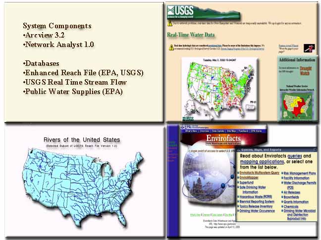
Figure 1. RiverSpill components and databases
William B. Samuels, Jonathan Pickus, David Amstutz, Rakesh Bahadur
A GIS-based tool has been developed to calculate the travel time (based on real-time stream flow measurements), decay, and dispersion of a pollutant introduced into a surface water. The tool allows the user to: select a location on a river to introduce a pollutant, track the pollutant downstream, under real-time flow conditions, to a water supply intake, further track the pollutant to a water filtration plant, and identify the overall population served by the plant. The tool requires two databases from USEPA and one database from USGS.
In cooperation with the Federal Emergency Management Agency (FEMA), the Technical Support Working Group (TSWG) has sponsored a project to develop a software program to assess the vulnerability of national waterways to terrorist threats, and other natural and manmade disasters, which may cause toxic pollution; plan for better protective measures; and assess and manage consequences of emergency incidents. The prototype system, RiverSpill has been developed and is operational for Ohio and Utah.
RiverSpill is a Geographic Information System (GIS)-based software tool with integrated data base capability that is used to track and model the flow and concentration of contaminants in the source waters (surface) of a public water supply. The system contains the following models and databases:
The databases required for this tool include the Enhanced River Reach File (ERF1), the USGS real-time stream flow measurements, and the EPA Safe Drinking Water Information System (SDWIS). The Arcview Network Analyst extension is used to integrate the databases and to provide the user with a tool to quickly assess the consequences of the introduction of a chemical or biological contaminant to the source waters (surface water) of a public water supply (see figure 1).
Figure 1. RiverSpill components and databases
The original EPA Reach File Version 1.0 (RF1) is a vector database of approximately 700,000 miles of streams and open waters in the conterminous United States. The RF1 stream flow data consist of mean annual flow and 7Q10 low flow estimates made at the downstream ends of more than 60,000 transport reaches. A 7Q10 low flow estimate is the lowest average flow, averaged over a period of seven consecutive days, within ten years of record. The digital data set ERF1 includes enhancements to the EPA's River Reach File 1 (RF1) to ensure the hydrologic integrity of the digital reach traces and to quantify the time of travel of river reaches and reservoirs. ERF1 was designed to be a digital database of river reaches capable of supporting regional and national water-quality and river-flow modeling and transport investigations in the water-resources community.
The stream-gauging program of the USGS is an aggregation of networks and individual stream flow stations that originally were established for various purposes. Approximately 5,000 of the 6,900 U.S. Geological Survey sampling stations are equipped with telemetry to transmit data on stream flow, temperature, and other parameters back to a database for real-time viewing via the World Wide Web.
The locations of public water supply plants and intakes were obtained from the EPA Safe Drinking Water Information System (SDWIS). The Safe Drinking Water Information System (SDWIS) contains information about public water systems and their violations of EPA's drinking water regulations. SDWIS is an EPA national database storing routine information about the nation's drinking water. The SDWIS stores the information EPA needs to monitor approximately 175,000 public water systems.
The integrated system calculates, locates, and maps the population at risk from the introduction of contaminants to the public water supply. The Real Time River Spill Model calculates the time of travel based on real time stream flow measurements, decay, and dispersion of a contaminant introduced into surface water. Prototype systems have been set up and tested for Ohio and Utah. The databases and software are directly extensible to the rest of the US. The GIS-based tool developed for this project consists of three primary components:
The following relationship seems to be a generally accepted form for relating velocity to flow:
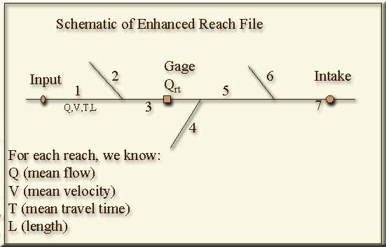
Figure 2. Schematic of the Enhanced Reach File and RiverSpill Network
The steps to calculate the time of travel, based on real time flow data are as follows:
The initial mass (Mo) of substance will be reduced to a secondary mass (M) using the temporal decay parameters assigned to that substance.
The distribution of a substance introduced to a river is governed by the convection-diffusion equations for turbulent flow (Taylor, 1954). The equations are simplified by assuming the molecular diffusion to be negligible, the density gradients are small compared with the concentration gradients, and the mass flux is proportional to the mean concentration and in the direction of decreasing concentration. The remaining terms represent the change in concentration of the substance with time, the convective mass transfer associated with the fluid velocity, and the turbulent mass transfer.
Further assumptions can be made by considering the concentration of substance to be a function only of time and along the stream dimension. The along stream velocity is considered constant (the average flow over the uniform cross section). These simplifying assumptions are wholly consistent with making use of the available data from the stream gauging stations. In summary, the assumptions arew as follows:
Modeling of river flow, and more especially the dispersion of substances within river flow, is a challenging task. The task is challenging because there are to few observations to support the equations representing the involved physics. Observations are lacking largely because of the complex stream geometries and variations in streambed characteristics. The difficulties in modeling river flow are summarized in several references (Novak, 1985).
The analytical model we use characterizes one-dimensional turbulent diffusion in constant density flow. The concentration is considered to be a function only of time and the distance along the longitudinal axis. Average velocities, calculated from real-time values reported from river gauging stations, are applied over the uniform cross sections. The initial condition specifies that a finite mass of substance is released instantaneously and uniformly over the cross section. Mathematically the initial release is from a Dirac delta function. The boundary condition specifies that the concentration remains zero for all time after release at infinite distances along the longitudinal axis (Ippen, 1966).
We can compare the model with the findings of a few carefully conducted dye studies and with documented pollution events. Results from the present model could also be compared with those from numerical models, where numerical models have been applied. Numerical models are finely tuned to the specific stretch of river to which they are applied. Therefore, one should not expect our generic model, which is being applied to all rivers, to yield results which agree in detail with the numerical models. If the models did agree then we would conclude that the numerical model was very likely not needed in the first place.Because the proposed model is to be applied throughout the United States, its skill must be assessed in the broadest sense. To accomplish this we selected rivers with a wide geographic distribution and with a variety of flow conditions. It is recognized of course that no single model will thoroughly address all of these circumstances. Nevertheless, our analysis was aimed at determining just how well or how poorly the model performed.
The US Geological Survey has assembled a large set of river observations (Jobson, 1996) which reflect the broad geographic distribution and widely varying flow conditions desired for model skill assessment. The data however, do not represent the most western and southwestern states. River observations reported by Jobson (1996) are tabulated in Appendices to the report and include original references. The observations represent 102 cases where dye was injected in 38 rivers. Multiple dye injections were made at the same, and in some cases, differing river locations. Dye injections were also made under varying flow conditions. From the variety of rivers investigated, 11 were selected for the model skill assessment study. The 11 were selected to meet the requirements for wide geographic representation (Hydrologic Regions), and varying flow conditions. Where possible, rivers with replicate dye injections were selected preferentially. The rivers used for skill assessment, are shown in Figure 3. The number of separate dye injections for each are: Amite (1), Antietam (6), Bighorn (2), Chattahoochee (2), Clinch (4), Embarras (3), Hoosic (1), Kaskaskia (3), N. Platte (1), Sabine (5), and Souris (6). Thus, 34 separate cases, representing 11 rivers are used in the river model skill assessment. The number of rivers and separate cases from each, used in the skill assessment, are considered appropriate to the purposes of the prototype model.
The observations provided by Jobson (1996) for each dye injection site include the distance(s) traveled, river discharge, time when dye began to arrive, time of arrival of the peak concentration, and time of arrival of the trailing edge of dye. For purposes of the skill assessment, the measured river discharge was compared with the historic discharge data in the River Reach Files to determine the coefficient "a" to be used to calculate river velocity.
Time of travel for the peak or central concentration was calculated for each reported stretch of river. Comparisons were made for observed and modeled travel times for the peak concentrations, versus distance traveled. The results are remarkably very good. For example, the modeled and observed travel times for the Antietam River are shown in figure 3. The results for the Amite River shows the convergence of the model and observed travel times with a subsequent divergence after 100 km distance.
The results from the comparison of observations and model output are summarized in the Regression Diagram of the observed and modeled peak concentrations . The regression diagram illustrates excellent agreement ( r = 0.87) between the observed and modeled data sets. The 34 separate cases, from the 11 rivers represent more the one hundred separate distances traveled (see figure 3).
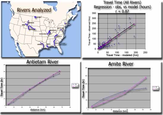
Figure 3. Model skill assessment - comparison of observed and modeled results
Figure 4 below shows the RiverSpill output for a hypothetical spill on the Maumee River in Western Ohio. Using the Network Analyst, "Find Closest Facility" function, the nearest gage to the spill site is determined. The URL for this gage is extracted from the gage attribute table and passed to an Internet Browser. The real-time flow and stage are displayed in the Browser window. In addition, the flow and stage data are extracted by a parsing program and passed to the flow-velocity algorithm mentioned above. The time-of-travel for each reach, based on the real-time velocity is calculated. The "Find Closest Facility" is invoked again, using the public water supply intakes as the facilities and the time-of-travel attribute as the cost field. Public water supplies along the flow path are displayed on the map and in an associated table. Personnel responsible for for operation of the water supply facilities, and their telephone numbers, are also identified in the table. If the concentration of the pollutant at the intake is above a specified level of concern, then the intake and its associated table record are colored red to indicate a warning.
A companion model, PipelineNet, has been developed to trace the path and concentration of toxic substances released from any point within a water pipeline network. PipelineNet has been applied sucessfully to Salt Lake City. Success with modeling a complex system such as exists in Salt Lake City, gives reason for optimism in applying PipelineNet elsewhere.
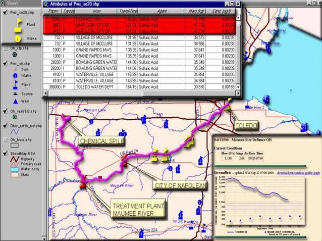
Figure 4. RiverSpill output for the Maumee River, Ohio
This project was funded by the Technical Support Working Group (TSWG), Infrastructure Protection (IP) sub-group. Martha Snyderwime is the TSWG program manager for the IP sub-group. Paul Bryant, Federal Emergency Management Agency was the government technical manager for this project. Dr. Walter Grayman, Consulting Engineer and Dr. Rolf Deininger, University of Michigan School of Public Health provided technical guidance to this project.
Ippen, Arthur T. Estuary and Coastline Hydrodynamics, Engineering Societies Monographs, McGraw-Hill Book Company, New York, 1966. 744pp.
Jobson, Harvey E. Prediction of Traveltime and Longitudinal Dispersion in Rivers and Streams, USGS Water-Resources Investigations Report 96-4013, 1996, 60pp.
Leopold, L.L. and T. Maddock, Jr., The Hydrologic Geometry of Stream Channels and Some Physiographic Implications, USGS Professional Paper No. 252, 1953.
Maidment, David, ed., Handbook of Hydrology, McGraw-Hill Book Company, New York, 1993.
Novak, P. (ed.) Developments in Hydraulic Engineering-3, Elsevier Applied Science Publishers, LTD. Essex, England, 1985, 316pp.
Taylor, G. I., Dispersion of Matter in Turbulent Flow through a Pipe, Proc. Roy. Soc. London (A), Vol. 223, 1954.
http://www.epa.gov/QUAL2E_WINDOWS Enhanced Stream Water Quality Model, Windows (QUAL2E)
http://baltimore.umbc.edu/mdnsdi/metadata/rf1.html, U.S. EPA Reach File 1 (RF1) for the Conterminous United States in BASINS, Metadata Record
http://www.epa.gov/owowwtr1/NPS/gis/reach.html, Office of Water River Reach Files
W.E. Gates and Associates, Inc., Estimation of Streamflows and the Reach File, Prepared for the U.S. Environmental Protection Agency, Monitoring Branch, Washington, DC.
http://water.usgs.gov/lookup/getspatial?ERF1, Enhanced Reach File Metadata Record
Kenneth L. Wahl, Wilbert O. Thomas, Jr., and Robert M. Hirsch, Stream-Gaging Program of the U.S. Geological Survey, U.S. Geological Survey Circular 1123, Reston, Virginia, 1995
SDWIS home page, http://www.epa.gov/OGWDW/datab/sfed.html