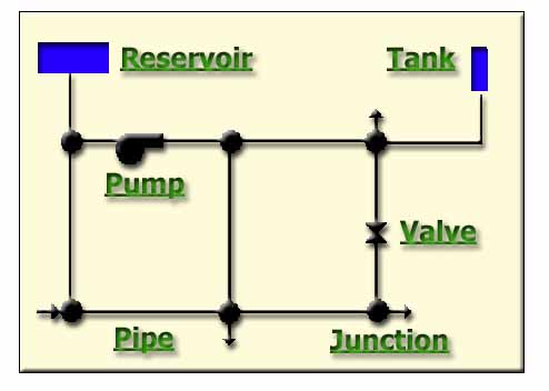
Figure 1. Schematic of Water Pipeline Network in EPANET.
Rakesh Bahadur, Jonathan Pickus, David Amstutz and William Samuels
This paper describes a project to integrate EPANET and Arcview to assist emergency managers in assessing the risks to public water supplies. The integrated system is called PipelineNet. This system calculates, locates, and maps the population at risk from the introduction of contaminants to the public water supply. The EPANET toolkit allowed Arcview to utilize the EPANET engine to route a contaminant through the system under extended period simulation. The results of the simulation are viewed within Arcview along with additional coverages representing population and infrastructure. The system was tested using the Salt Lake City database composed of approximately 31,000 links and 52 pressure zones.
In cooperation with the Federal Emergency Management Agency, the Technical Support Working Group (TSWG) has sponsored a project to develop software programs that would estimate the consequences of a terrorist attack on a city’s drinking water infrastructure. The prototype system, PipelineNet, has been developed and is operational for Salt Lake City, UT.
PipelineNet is a Geographic Information System (GIS)-based software tool with integrated data base capability that can be used to model the flow and concentration of contaminants in a city’s drinking water pipeline infrastructure. It contains a pipe network hydraulic model (EPANET), maps, and a US Census Population database. The PipelineNet model estimates the population at risk due to the introduction of contaminants in the public water supply and graphically maps this population. The PipelineNet model permits the user to model the flow and concentration of a biological or chemical agent within a city or municipal water system. This model assesses the effects of water treatment on the agent, models the flow and concentration of an agent through the water distribution system within a city or municipality, and calculates the population at risk. PipelineNet performs the following functions:
The system is designed for:
The EPANET component of PipelineNet was developed by the Water Supply and Water Resources Division (formerly the Drinking Water Research Division) of the U.S. Environmental Protection Agency's National Risk Management Research Laboratory. EPANET performs extended period simulation of hydraulic and water quality behavior within pressurized pipe networks. A network can consist of pipes, nodes (pipe junctions), pumps, valves and storage tanks or reservoirs (see figure 1). EPANET tracks the flow of water in each pipe, the pressure at each node, the height of water in each tank, and the concentration of a chemical species throughout the network during a simulation period comprised of multiple time steps. In addition to chemical species, water age and source tracing can also be simulated. EPANET can perform complex hydraulic modeling based on numerous variables and water system components. The system also features a full featured and accurate hydraulic modeling capability, and water quality modeling capability. EPANET can also be used to study such water quality phenomena as the blending of water from different sources, age of water throughout a system, loss of chlorine residuals, growth of disinfections by-products, and contaminant propagation events.
Figure 1. Schematic of Water Pipeline Network in EPANET.
The Windows version of EPANET provides an integrated environment for editing network input data, running hydraulic and water quality simulations, and viewing the results in a variety of formats. These include color-coded network maps, data tables, time series graphs, and contour plots. Figure 2 shows the EPANET windows interface and example output.
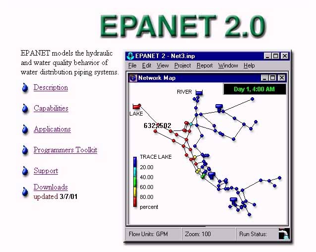
Figure 2. EPANET windows interface and example output.
A key part of the PipelineNet development is the capability to trace the impacts of a contaminant in a distribution system. There are many existing software programs that perform the technical task of modeling water quality in a distribution system including the very popular EPANET model that is being used as part of the present project. There are two modes of operation of a distribution system model, steady-state and extended period simulation (EPS). Whereas, steady state analysis is frequently used for some hydraulic analyses (master planning, fire flow requirements), extended period simulation is essential for any meaning water quality analysis. There are two primary reasons why extended period simulation (EPS) is necessary when doing water quality modeling:
Salt Lake City (SLC) has been selected as the demonstration system for the project. The Salt Lake City Department of Public Utilities has a very detailed steady state model (around 30,000 pipes) of their system that was developed for them by a consulting engineer in 1995 (see figure 3). Because of the reasons outlined above, in order to use the model for tracing water quality contaminants, it is necessary to convert this model to extended period simulation. A three-phase approach to developing an EPS capability for Salt Lake City is outlined below.
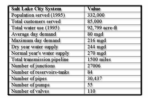
Figure 3. Summary of the Salt Lake City steady state model.
In this phase, a rudimentary EPS representation of the SLC system was developed in order to demonstrate the prototype software being developed as part of the project. This rudimentary EPS model made the following assumptions: (1) demands and system operations do not change over the course of the day and reflect the maximum day or peak hour conditions of the current steady-state model; and (2) all tanks and reservoirs can be represented in the model as infinite sized basins. The latter assumption is consistent with the assumption that is made in all steady state modeling. The consequence of the first assumption is that the effects of temporally varying demands and operation will not be reflected in the resulting model applications. More seriously, the consequence of the second assumption is that a contaminant that enters any tank or reservoir in the distribution system will be instantaneously disappear because of the complete dilution by the infinite sized basin. Examination of the impacts of these assumptions on EPS modeling of Salt Lake City indicate that the resulting model will provide only a poor approximation of the actual movement of a contaminant through the system but will be usable to demonstrate the prototype software.
Figure 4 shows an example of this form of calibration. A comparison is made between the obesrved and modeled water level in a tank. The difference in results is between 1 and 2 feet. The results of phase II is an EPS model of the system as it is expected to operate during the Olympic period in 2002.
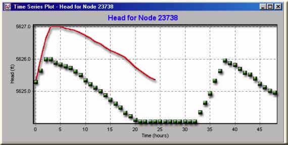
Figure 4. Comparison between observed and simulated water level for Tank # 23738 (White Reservior).
The primary limitation of the Phase II model is that it will be "hard-wired" to only represent conditions as they are expected to occur during the Olympic period. Though this should be adequate to operate the model during that period and to simulate the introduction of a contaminant at any location, it could not be used directly to model EPS conditions during other periods. During different periods, demands change and the basic operation of the system can vary significantly. For example, operations during the summer usually differ greatly from winter operation. Typically, some tanks may be taken out of service or their levels lowered. In Phase III, the model would be expanded to represent demands that are representative of different seasons and would represent different operating policies. Since "hard-wiring" operations will not provide this flexibility, it is necessary to define the operation by a series of rules that can be incorporated into the model. For example, these rules may relate the pump operation to the water levels in tanks or describe when valves are opened or closed based on other conditions. Development of such rules in a system as complex as Salt Lake City will be a challenge. It will require significant interaction with SLC operators and engineers in order to define the operation of the system.
The result of this task will be a very robust EPS representation of the Salt Lake City distribution system. In addition to supporting the model for use in emergency contamination cases, the model can serve as an extremely usefull tool to SLC to test alternative operations and designs, to study impacts on water quality, and to reduce energy costs.
A process flow diagram showing the ARCVIEW and EPANET integrated model, PipelineNet, is shown in figure 5. The integration is accomplished using EPANET Toolkit, and GUIs written in Visual Basic and ARCVIEW programming language (avenue). PipelineNet has been developed with several custom tools and features for hydrological oriented environmental decision support. The whole system runs through a series of GUIs. PipelineNet is developed with several custom tools and features to provide an interface with EPANET. The input file is prepared before starting PipelineNet except the source and the injection. PipelineNet follows all of EPANET conventions.
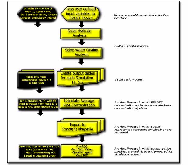
Figure 5. Process flow diagram showing EPANET - Arcview Linkage
A single click on the map anchors the point and initiates the EPANET Source Point Parameters GUI as shown in figure 6. This selects the node where injection will occur. Injection units follow EPANET rules, negative demand nodes can have mass/volume and positive demand nodes can have mass/minute. Initialize Input Parameters Button is selected the very first time running the EPANET interface. Once the Source Point is properly selected, Set Source starts the EPANET analysis. The user can verify the input parameters in the popup window that follows. When PipelineNet is finished processing, the resulting hourly simulation concentrations will automatically load in< the View and can be displayed using the Pipeline View Parameters GUI.
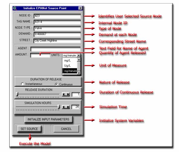
Figure 6. PipelineNet User Interface
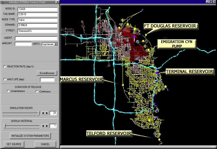
Figure 7. Example PipelineNet Output.
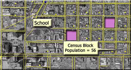
Figure 8. PipelineNet overlay with aerial photography and schools.
The PipelineNet simulates the flow and concentration of biological or chemical contaminants in a city or municipality's water distribution system. The integrated model is a powerful tool for routine planning and emergency response. It gives emergency managers real time information for estimating the risks to public water supplies and population at risk. The PipelineNet can calculate, locate, and map the population at risk from the introduction of contaminants to the public water supply.
Rossman, L.A., 2000. EPANET 2 User's Manual, National Risk Management Research Laboratory, Office of research and Development, USEPA, EPA Publication EPA/600/R-00/057, September, 2000. 200 p.
Esri, 1994, ARCVIEW User's Manual, Environmental Systems Research Institute, Redlands, CA, 98 p.
SLC, 1995, Water Planning Master Plan. Salt Lake City Department of Public Utilities, Salt Lake City, Utah.
This project was funded by the Technical Support Working Group (TSWG), Infrastructure Protection (IP) sub-group. Martha Snyderwime is the TSWG program manager for the IP sub-group. Paul Bryant, Federal Emergency Management Agency was the government technical manager for this project. The authors gratefully acknowledge the cooperation of the Salt Lake City Department of Public Utilities, particularly Tom Ward, Chuck Call, and Nick Kryger. Dr. Walter Grayman, Consulting Engineer and Dr. Rolf Deininger, University of Michigan School of Public Health provided technical guidance to this project.