Desktop and Internet GIS Development for Spatial Segregation Analysis

David W. S. Wong

Several geographical measures of segregation have been introduced in the past decade. Because they require certain types of spatial information in their formulations, it is natural to incorporate these spatial measures in a GIS environment. This paper documents an effort in using Avenue scripts in ArcView to implement a set of spatial segregation measures. The results of this development (project files) are available for researchers and practitioners. In addition, segregation is often a concern of local communities. Given the wide-spread access of Internet, tools and data for analyzing spatial segregation are made accessible to the public through Internet GIS.

1. Introduction

Most studies on ethnic and residential segregation so far have relied heavily on the dissimilarity index D advocated by sociologists Duncan and Duncan (1955). Regardless of how useful it is in measuring the evenness dimension of segregation (Massey and Denton, 1988), it fails to distinguish population patterns effectively. A set of spatial segregation measures has been proposed during the past decade, however, these measures have not been used extensively. Part of the reason that spatial measures were not widely adopted is because they were no existing tools to compute these measures. Generic tools such as database programs and spreadsheets cannot handle the computation because spatial information is needed in the calculation. Therefore, using GIS is necessary to develop such tools. However, accessibility to desktop GIS technology, though improved over the last decade, is still not high outside of the academic and research communities. Even if tools for computing spatial segregation are developed using GIS, local communities and public organizations will still be inaccessible to the tools and technology. There is a need to make these tools to compute spatial segregation more accessible to the public, probably through Internet.

The purpose of this paper is to report a recent effort to implement a set of spatial segregation measures within ArcView GIS. These measures are developed as additional spatial analytical tools in the ArcView user interface. Interested users can download the project file (.apr) with the tools embedded from the website managed by the author ((http://geog.gmu.edu). In addition, this paper explores the possibility of delivering the tools to compute spatial segregation indices on Internet through ArcIMS such that the public can compute segregation measures for the areas they are interested in. The next section provides an overview of the set of spatial segregation measures. The third section discusses the implementation of these measures in ArcView GIS. Then, a framework to deliver the segregation analysis environment through Internet is proposed. It is followed by a summary and discussion section.

2. Spatial Segregation Measures

2.1. Two-group Measures

The most commonly used segregation measure is the dissimilarity index D advocated by Duncan and Duncan (1955). This index is easy to compute, and ranges from 0 to 1, indicating no segregation to perfect segregation, respectively. The specific definition of the index cannot be found in Equation (1) in Appendix 1.

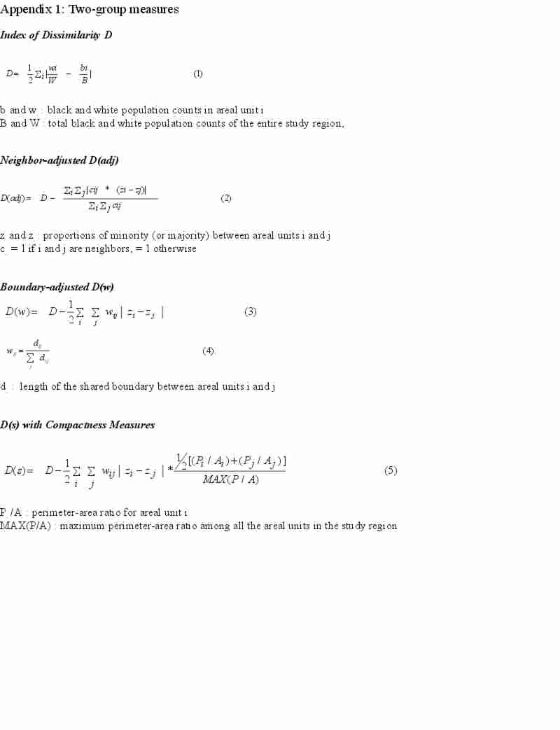
A major deficiency of D from a spatial perspective is that it cannot solve the checker-board problem. As long as each areal unit within the study area is dominated by one group or the other exclusively, the D index will return a "1", indicating a perfectly segregated situation, even if some adjacency areal units are occupied by different groups. Rearranging populations among areal units will not change the D value because D as well as other traditional measures are aspatial measures.

To overcome this limitation, spatial versions of D were proposed. The D(adj) index introduced by Morrill (1991) is the original dissimilarity index less the amount of interaction across areal unit boundaries. The level of interaction between any pair of neighboring units is then determined by the differences in the racial mixes of neighboring units. D(adj) is formally defined in Equation (2) in Appendix 1. This measure was further modified by Wong (1993) in several directions. Based upon the premise that the intensity of interactions across a boundary is not a simple function of adjacency, but likely the length of the shared boundary, the D(adj) index is slightly rewritten to incorporate a boundary-length component to moderate the interactions across areal units. This index, labeled as D(w), is defined in Equations (3) and (4) in Appendix 1. Furthermore, Wong (1993) argued that the intensity of interactions between areal units is also a function of the size, shape, or the compactness of the two adjacency areal units. To incorporate the geometric characteristics of areal units into the measures of segregation, a compactness measure based upon the perimeter-area ratio was used. Equation (3) is further modified to formulate the index D(s), which is defined in Equation (5) in Appendix 1.

2.2. Multi-group Measures

The study of segregation in North America has been dominated by the two-group model as blacks and whites have been the dominant groups historically. However, recent immigration history has made the North America societies more multiethnic. Therefore, there is a need to measure segregation in multi-ethnic settings. Based upon the concept of the dissimilarity index D, Morgan (1975) and later Sakoda (1981) introduced a multi-group version of D. It's definition, D(m) is in Equations (1) and (2) of Appendix 2.

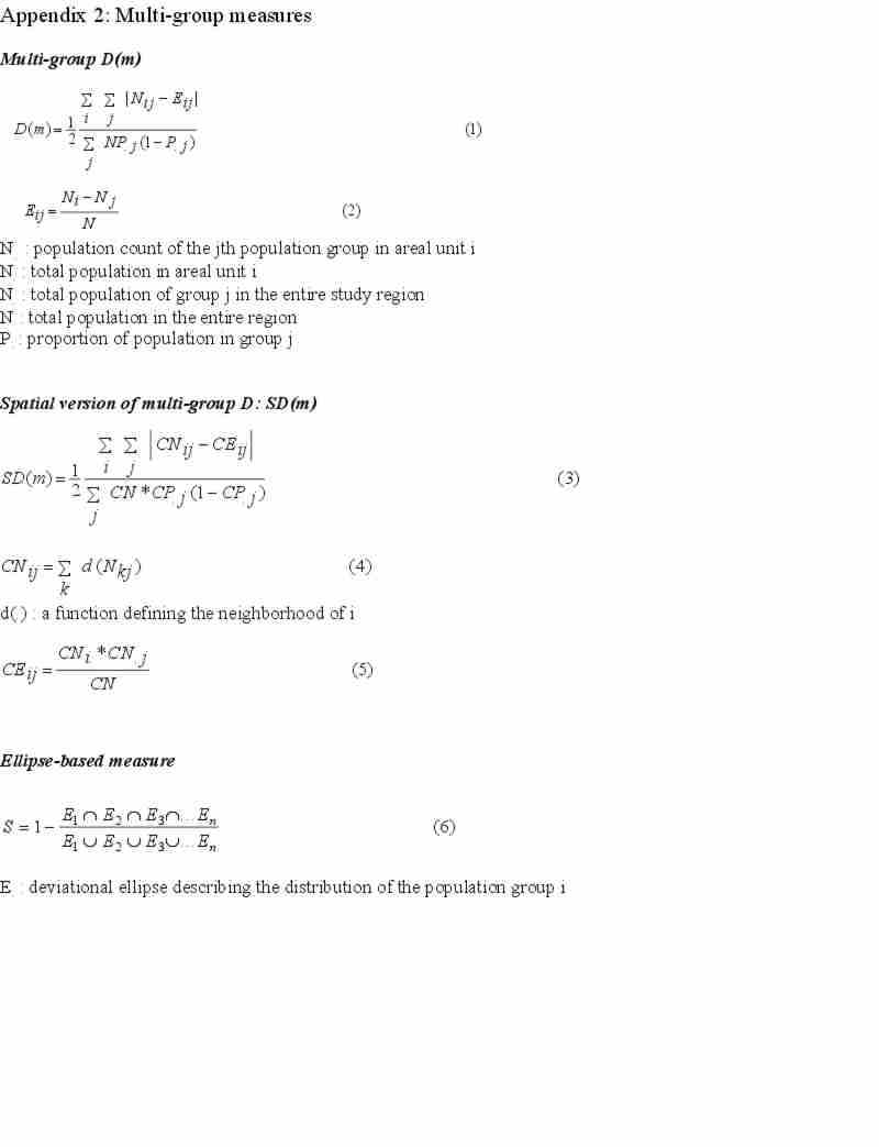
This multi-group measure of segregation can accommodate more than two groups, but shares the same limitations with the dissimilarity index D. That is, the measure is aspatial and rearranging populations among areal units will not change the overall level of segregation. To inject the spatial dimension into this multi-group measure, a spatial version was proposed (Wong, 1998). The formulation of the spatial version of D(m) is based upon the concept of composite population counts. The composite population count of areal unit i for group j is defined in Equation (4) of Appendix 2, which is based upon the premise that within the neighborhood of i, people belong to different ethnic groups can interact as if they are in unit i. After the composite population counts for all areal units are computed, they are used to calculate D(m) as if they are the original population counts. Therefore, the spatial version of D(m) is SD(m) as defined in Equations (3) and (5) of Appendix 2. The major difference between the D(m) and SD(m) is in the population count. Using the composite population counts in SD(m) accommodates the interactions of population groups within the neighborhood, which are not accounted for in the conceptualization of D(m). Therefore, D(m) and SD(m) have the same mathematical properties.

Based upon the concept of spatial congruence, an ellipse-based measure was suggested to evaluate spatial segregation (Wong, 1999). Given the locations of people of a given group, an ellipse is used to fit the locations to capture the overall spatial distribution characteristics of the group. After multiple ellipses are derived for different groups, they are then overlaid to derive an index of segregation based upon the ratio of the intersection and union of all ellipses. Mathematically, the S index is defined in Equation (6) in Appendix 2.

3. Implementation of Spatial Segregation Measures

GIS are useful in segregation studies in general (Wong, 1996). However, most analysts of population and segregation studies probably take advantage of only the mapping capability of GIS without fully exploiting the potential of GIS in assisting population and segregation studies. One definite potential of GIS is to support spatial analysis. However, most standard spatial analytical functions in GIS fail to support the types of index calculation described in the previous section. Still GIS can play a critical role in the computation of any spatial measures, including the set discussed above by providing or deriving spatial information necessary for the calculation of spatial measures.

A previous effort in using GIS to implement spatial measures of segregation has been successful (Wong and Chong, 1998). However, that implementation exercise was not very efficient and rather costly because it had to rely on a GIS package (pre-Arc/Info 8 versions) and S-Plus, a statistical modeling package. In addition, the process was not a GIS process in the sense that it requires using only database functions to search through the Polygon Attribute Table (PAT) and the Arc Attribute Table (AAT) to derive most of the spatial information required.

With the goal to maximize the number of potential users and minimize the cost of using these spatial segregation measures, ArcView was chosen as the GIS platform to implement the spatial measures. Besides its relative user-friendliness and popularity among GIS users and social scientists (sociologists, economists, political scientists and planners), several characteristics of ArcView, including the powerful OO programming environment with Avenue, customizable GUI, the use of more compacted non-topological shapefiles, make it a desirable candidate for the implementation. Even though shapefiles data structure does not stored topological information in the database (Burrough and McDonnell, 1998), but given the object-oriented environment in ArcView, topological information, geometric characteristics and spatial relations among geographic features can be computed quite efficiently.

3.1. Two-group Measures

All two-group measures consist of two major components: the traditional D dissimilarity index, and the spatial component which moderates D. The computation of D is rather straightforward because it requires only the population data which are usually stored in the feature attribute table. An algorithm written in Avenue scripts was developed to calculate the traditional D index without using any spatial operation in ArcView.

To compute the spatial component, several items are needed to derive from GIS in addition to the population data. Adjacency is used to compare the differences in ratio mixes. To identify neighbors of a given areal unit in ArcView, conceptually it is the same as to identify areal units with distance = 0 to the referenced areal unit. Specifically, in the ArcView environment, first the referenced areal i is selected. Then, issuing the SELECTBYTHEME request to the theme and set the selection type to #FTAB_RELTYPE_ISWITHINDISTANCEOF with a distance of "0", areal units in the theme adjacent to i, or with a distance of zero from i, will be selected. This selection process essentially executes the c_ij element in Equation (2) in Appendix 1 and permits the comparison of attributes of neighboring units in Equations (3), (4) and (5) in Appendix 1. By changing the distance parameter of the SELECTBYTHEME request, the neighborhood definition becomes flexibly enough to accommodate other criteria besides the adjacency criterion.

When neighbors of i are selected, geometric parameters or attributes of i and each of its neighbors are derived. Perimeters (P_i and P_j) of each polygon pair can be obtained by sending the request RETURNLENGTH to the polygon objects. Similarly, the areas (A_i and A_j) of the polygon pair can be obtained by sending the request RETURNAREA to the polygon objects. After obtaining the perimeter and area information, the compactness measure (P/A) can be derived. In order to identify the line segment or segments representing the share boundary of the two polygons, the request LINEINTERSECTION can be issued to the two polygons i and j. This request will return the intersecting line segment or segments of the two adjacent polygons. By issuing the RETURNLENGTH request again to the common boundary line object, d_ij is then extracted.

Regardless whether adjacency information (c_ij in Equation (2) of Appendix 1) or the length of a shared boundary (w_ij and d_ij in Equations (3) and (4) of Appendix 1) is needed, the information can be stored for later access. Perimeter and area measures of each polygon can be stored as additional items in the feature attribute table to be used in later computation. However, storing and retrieving these different types of spatial information in tables are not very efficient. First, storing these tables or matrices, especially for large spatial systems, will occupy a lot of memory space and in turn will slow down the computation. Second, accessing tables in ArcView is not a very efficient process. Instead of using the traditional approach to store all types of spatial information in tables, the current approach is to take advantage of the efficient spatial indexing system which provides very efficient spatial selection operations.

Basically, the operation proceeds from one polygon to the next until all polygons are enumerated. In detail, the operation includes the following major steps:

1) select a polygon i in the study area.

2) select neighbors of i (i.e., j).

3) between i and each j, derive the racial mixes (z_i and z_j), and their absolute differences. This

step will produce the numerator of Equation (2) for D(adj).

4) derive the perimeter and area for each neighboring pair. This step permits the computation of the numerator of the last part of Equation (5) for D(s).

5) given perimeter information, intersection operation on neighboring polygons is used to derive the shared boundary to compute d_ij and w_ij in Equation (4) and for D(w). 6) select another polygon in the study area to repeat Steps #2 to #5 until all polygons are enumerated.

7) select the MAX(P/A) from P/A ratios for all polygons.

8) compute the spatial components for D(adj), D(w) and D(s), and then subtract them from D.

In addition, the algorithm also allows users to use another MAX(P/A), which is likely the global MAX(P/A) among all study regions, to compute D(s). The D(s)'s based upon the global MAX(P/A) provide meaningful comparison of segregation levels among regions with different spatial partitioning characteristics (Wong, 1993). After the spatial components of spatial measures are computed, they are subtracted from the aspatial measure D.

3.2. Multi-group Measures

The implementation of the spatial version of the multi-group dissimilarity index is very similar to the two-group spatial measures. The key process is to derive the composite population count for a population group in each areal unit (Equation (4) in Appendix 2). A composite population count is defined by a neighborhood function. For each areal unit i, neighboring units are selected using the theme selection request as in the two-group implementation process. Then the composite population counts for different groups are derived for the referenced areal unit i by aggregating population counts in the referenced unit and surrounding areal units for each group. Composite population counts are then derived for all population groups in all areal units. Based upon the computed composite population counts, rows and columns non-spatial operations for tables are used to compute SD(m) in Equation (3) in Appendix 2.

For the multi-group ellipse-based segregation index, the process is quite different from previous indices. To fit an ellipse to the spatial distribution of a population group, the first step is to extract the x-y coordinates of each areal unit or population point. Because the calculation of an ellipse is entirely based upon the x-y coordinates of the point locations or centroids of polygons, therefore, for each polygon unit, the centroid as a point is first derived by issuing the RETURNCETER request to the polygon and its x-y coordinates are extracted using the GETX and GETY requests issued to the centroid point. Because each polygon or point location may have different population counts or weights, these weights or counts are then multiplied to the coordinate readings. For each population group and based upon the locations (x-y coordinates) of the population group, four parameters of the ellipse are derived. These four parameters are the center (in terms of x-y coordinates), the two lengths of the perpendicular axes, and the angle of rotation of the ellipse. These parameters serve as input to create the ellipse object in ArcView (E_i). After an ellipse is created for each population group, it is converted into a polygon object for subsequent operations which support polygon shape objects but not ellipses. Intersection of ellipses is obtained by the request RETURNINTERSECTION issued to the two corresponding polygon objects. Similarly, union of ellipses is obtained by the request RETURNUNION issued to the two corresponding polygon shapes. These steps are repeated for all ellipses to obtain the intersection and union of all ellipses. Then requests are sent to the intersecting polygon and the union polygon to obtain the areas in order to derive the numerator and denominator of Equation (6) in Appendix 2 and thus compute the S index. The algorithm provides the option for users to store the ellipses as polygons for all population groups into shapefiles, and store the intersection and union as polygons for display to provide a visual impression of the segregation level.

Algorithms developed include the traditional measures of segregation for two-group and multi-group situations (D and D(m)), spatial measures for the two-group cases (D(adj), D(w), and D(s)), spatial measure for multi-group cases (SD(m)), and the ellipse-based measure for multi-group cases. Scripts written to implement these algorithms are compiled and are linked to new menu items under a new menu labeled as "Segregation" in the ArcView GUI (Figure 1). These new functions and their corresponding items in the ArcView GUI are saved in a project file. Under the new menu, four items corresponding to the four scripts for the algorithms are added. Interested users can download the project file from the website managed by the author (http://geog.gmu.edu/seg). An example using the ellipse-based S index on population counts of white and black for counties in Georgia is also shown in Figure 1.

4. Internet Extension of Spatial Segregation Analysis GIS

Levels of segregation are of great concerns in public policy formulation and analysis. Besides academics and policy makers, local residents, community activists, and political leaders are likely concerned about the level of segregation at the community or neighborhood levels. Even though GIS technology has proliferated tremendously in different levels of the society, the majority people of the nation still do not have access to the technology. In order to make available the spatial segregation analytical tools to the public, delivering the tools and data through Internet probably is the most desirable. Therefore, the enhanced ArcView functions for spatial segregation measures have to work through the Internet environment. This model can be generalized to increase the public access to other spatial analytical tools that are supported by GIS in general and ArcView in specific.

There are many possible approaches to port these spatial functions to the Internet environment. On one extreme, all codes for these functions together with other GIS capabilities, such as basic spatial query and selection and cartographic displays, could be rewritten in codes supported by the Internet environment. This approach starts from scratch and will result in a very efficient and highly specialized environment. A definite difficulty is that it is costly in development. The other extreme is to rely on existing resources to minimize development effort. That is to couple existing tools or packages to deliver the segregation computation capability to the clients on Internet. The rest of this paper discusses a preliminary framework to explore this later approach.

The computational tools developed on ArcView are based upon Avenue, which is not a standard tool in today's development environment. Esri has been advocating Visual Basic for Applications (VBA) which will work with ArcInfo8 and ArcGIS. To utilize the new GIS technology with VBA, all Avenue scripts have to be converted. As the strategy is to minimize development effort, it is preferred to have the computation tools remained in ArcView 3.X. In terms of the web interface, several Esri products offer different options. ArcView IMS probably will work best in this case, but unfortunately Esri has indicated to discontinue the support of this product. MapObjects IMS can offer the most flexibility, but it requires more development effort. Also, similar to ArcView IMS, MapObjects will not be the focus of Esri future development effort. On the other hand, Esri has been promoting ArcIMS as the Internet product to deliver maps and spatial data on the web. Therefore, the development strategy is to couple ArcIMS and ArcView 3.X together.

Figure 2 is the user front end based upon the conceptualization of the development model. This front end inserts an ArcIMS page on the right with clients' inputs on the left. There are three main components. The ArcIMS page on the right allows clients to select areas from different data layers. It serves the spatial query function. The second component is for clients to select population groups from which spatial segregation measures are derived. The third component is to indicate what aspatial and spatial measures are requested by the clients. After all these selections were made, information is transmitted back to the server through different channels for processing.

After the client selects the interested area for the analysis by interacting with the map rendered by the ArcIMS server, the selection information is passed back to ArcIMS. On the ArcIMS server, the extract server is setup to subset the selected features from the corresponding shapefiles. The shapefiles of the selected features will be created on the web server (Figure 3). After the client chooses the population groups and the index or indices for the analysis, these selection parameters are written into a text file document on the web server.

Next, the ArcView project file with the enhanced spatial segregation computation capability is modified such that when the file is triggered, it will automatically retrieve parameter information from the parameter document and also the shapefiles extracted for the subset of features. ArcView will use the information stored in the parameter file to determine which population groups are used and which index or indices are computed. Then the results are posted back to the client.

However, implementing this framework encountered several obstacles. First, when the extract server extracts the selected features from the shapefiles, the shapefiles subset will be in compressed format. The file has to be uncompressed before ArcView can access the data and process the requests. Second, after the selection parameters are passed back to the server to create a document, ArcView has to be triggered. It is not clear how ArcView can be triggered. CGI/Perl is a promising option which has yet to be tested thoroughly. Third, when ArcView should be triggered to access the parameter file and the shapefiles subset is not clear. Because the shapefile subset and the parameter document are created through different processes that are not synchronized, it is possible that when ArcView was triggered, only one document was created. Finally, without using ASP, it seems to be difficult to pass the results from ArcView back to the client when ArcView finishes its computation. More research and development are needed to overcome these obstacles or to formulate a new framework to develop a spatial segregation analysis module on the web.

5. Summary

This paper provides a concise overview of spatial segregation measures and documents how these measures were implemented in ArcView using Avenue. A project file with all tools for computing spatial segregation measures is available to the public (http://geog.gmu.edu/seg). The paper also proposes a framework to develop a web user front end for the spatial segregation GIS. Currently, the least-development effort approach was used by coupling ArcIMS and ArcView to minimize coding development. However, several major obstacles exist. Some of these obstacles may be removed with more research, but it is possible that another framework which requires more intense development effort has to be formulated.

There are several lessons that we can learn from the later part of this paper. The issue is how spatial analytical techniques in general can become accessible through the web environment. The approach adopted by most system developers these days is hardcore coding. It is possible to develop web-enabled programs to perform spatial analysis and these programs will perform efficiently in the web environment. However, taking this approach implicitly separates GIS applications and development on the web from the desktop. Numerous powerful tools, including the spatial segregation measures reviewed in this paper, have developed on desktop GIS. With efficient spatial indexing systems and spatial data models, desktop GIS can perform spatial queries and selections quite efficiently. These are essential building-block functions for many spatial analytical techniques developed on desktop GIS. With the intent to take advantage of the efficient spatial selection capability in desktop GIS, this paper explores the approach to rely on enhanced desktop GIS tools to perform spatial analysis while input information is gathered from users through the web interface. Unfortunately, this experiment has not been successful. It is true that many spatial analytical functions can be implemented on the web environment with programming, however, these functions will not perform as efficiently as those found on the desktop environment unless GIS data formats and models used in the web environment are comparable to those used on desktop environment. Currently, it seems that there is a big gap in the development of spatial analytical capability between the desktop and web environments.

Acknowledgment:

This project is partially supported by the National Institute of Health/Child Health and Human Development (NICHD) under the National Institute of Health (NIH) grant number 1 R03 HD38292-01.

Appendices

References

Burrough, P. A. and McDonnell, R. A. (1998). Principles of Geographical Information Systems. Oxford: Oxford University Press.

Duncan, O.D. and Duncan, B. (1955). A methodological analysis of segregation indexes. American Sociological Review, 20, 210:217.

Massey, D.S. and Denton, N. A. (1988). The dimensions of residential segregation. Social Forces, 67, 281-315.

Morgan, B.S. (1975). The segregation of socioeconomic groups in urban areas. Urban Studies 12: 47-60.

Morrill, R. L. (1991). On the measure of geographical segregation. Geography Research Forum, 11, 25-36.

Sakoda, J. N. (1981). A generalized index of dissimilarity. Demography 18: 245-250.

Wong. D.W.S. (1993). Spatial indices of segregation. Urban Studies 30: 559-72

Wong, D.W.S. (1996). Enhancing segregation studies using GIS. Computers, Environment and Urban Systems, 20(2), 99-109.

Wong, D.W.S. (1998). Measuring multiethnic spatial segregation. Urban Geography 19: 77-87

Wong, D.W.S. (1999). Geostatistics as measures of spatial segregation. Urban Geography 20(7): 635-647

Wong, D.W.S. and Chong, W. K. (1998). Using Spatial Segregation Measures in GIS and Statistical Modeling Packages. Urban Geography 19(5): 477-485.

David W. S. Wong
Associate Professor
Department of Geography
George Mason University
Fairfax, VA 22030
U.S.A.
Tel: 703-993-1212
Fax: 703-993-1216
Email: dwong2@gmu.edu