Assessment of Kriging Accuracy in the GIS Environment
Peter P. Siska and I-Kuai Hung
ABSTRACT
The demand for spatial data is on the rise. However, even the latest technology cannot guarantee an error free database in Geographic Information System (GIS). In natural resources the point field sampling is often used for spatially oriented projects and interpolation methods are implemented to predict the values in an unsampled location and to generate maps. In order to evaluate the performance of Kriging interpolation in GIS the Kriging errors were analyzed and compared to the four other interpolation methods using fundanmental statistical parameters. The sensitivity of ordinary Kriging interpolation in the GIS environment was evaluated with respect to the resolution of the predicted grid and conclusions were drawn for applications in spatial analysis.
METHODOLOGY AND DATA
Interpolation methods estimate the values in unsampled locations. The mapping and spatial analysis often requires converting the field measurements into continuous space. Therefore the point data sets must be converted to a continuous form using an interpolation method. The errors, however, enter the spatial database long before any interpolation method is applied to the data set. The first type of error is associated with sampling design. The magnitude of a sample, as well as the procedure of obtaining it, depend on the objectives of the sampling process, and consequently vary with these objectives (9). Increasing the sample size also improves the accuracy of measurements up to a certain point. In spatial analysis the sampling is often performed on a regular grid or on an irregular set of points however, this might not depict the true variation of studied phenomena in the space.
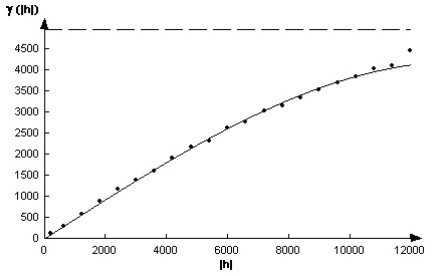
Figure 1.Variogram from Piloncillo data
The stratified random sampling is often recommended for spatial analysis (2). Unfortunately, it is not always possible to precisely follow the demands of the prescribed sampling methods. Therefore, the errors emanating from sampling design pollute the database and distort the true representation of the variation of studied phenomena before any measurements of spatial variable occur. The second group of errors arises from measurements and laboratory analysis. There is usually more than one way the measurement can be obtained. The difference between two measured values of the same quantity is called discrepancy (12). Discrepancies and sampling errors can be evaluated in spatial analysis by variograms. The nugget effect is determined by the intercept of the variogram curve with the vertical coordinate. Theoretically, the nugget effect should be zero, but due to the previously mentioned errors the nugget effect is usually greater than the zero value. Majority of variogram models have a significant nugget effect and therefore the small scale variation and noise in the data can be seen from the variogram models. However, this is not the case with the Piloncillo data used in this analysis. As Figure 1. indicates there is no nugget effect present in this data; both experimental and theoretical variograms have the origin in zero.
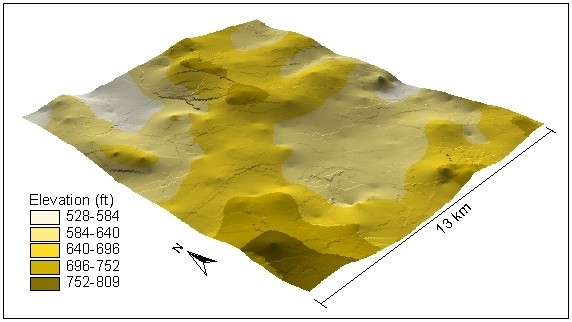
Figure 2.Piloncillo Surface from Ordinary Kriging Interpolation
There are a number of interpolation methods available (8) but one of the most frequently used interpolation method in GIS is Kriging (Figure 2). Kriging is an optimal interpolator offering a minimum error variance. The objective of this paper was to test Kriging interpolation within the GIS environment for accuracy. In this paper Kriging was applied to a low vacillating elevation data set and the errors from Kriging were evaluated using fundamental statistical parameters such as root mean square error, variance of errors, mean absolute error, etc. In addition, the Kriging errors were compared between two different software systems. The error propagation by interpolation method is difficult to identify since the bias associated with the sampling strategy and experimental error are difficult to measure. The Kriging errors have rarely been studied. Bancroft and Hobbs analyzed the distribution of Kriging errors based on deviation from normal distribution (1). Siska and Maggio (11) indicated the impact of surface dissectivity on a magnitude of Kriging errors and Siska and Hung (10) compared Kriging errors from GIS to the Kriging errors that arose from a geostatistical software at different grid resolutions.
RESULTS
The root mean square error (RMSE) is frequently used as an important parameter that indicates the accuracy of spatial analysis in GIS and remote sensing. The forty errors from the trend surface, Thiessen polygons, TIN (Triangular Irregular Network), IDW (Inverse Distance Weighted method). Kriging (Idrisi (3) and Arc-Info (4) environments) were analyzed and RMSE was calculated for each interpolation method. RMSE was calculated using the formula as Equation 1;
 -----(1)
where SSE is sum of errors (observed - estimated values) and n is the number of pairs (errors).
The results based on RMSE indicated that the interpolation using Triangular Irregular Network (TIN) yielded the smallest errors while the trend surface analysis indicated the highest RMSE. TIN interpolation was four times more accurate than the trend surface (the fitted model for the trend surface was as expressed in Equation 2) and 1.7 times than Inverse Distance Weighted (5) method, which performed less accurately than the Thiessen polygon method (Figure 3).
-----(1)
where SSE is sum of errors (observed - estimated values) and n is the number of pairs (errors).
The results based on RMSE indicated that the interpolation using Triangular Irregular Network (TIN) yielded the smallest errors while the trend surface analysis indicated the highest RMSE. TIN interpolation was four times more accurate than the trend surface (the fitted model for the trend surface was as expressed in Equation 2) and 1.7 times than Inverse Distance Weighted (5) method, which performed less accurately than the Thiessen polygon method (Figure 3).
 -----(2)
Interestingly enough the results indicated also a small difference between the software packages; the Kriging in Indrisi performed slightly better than the one in Arc/Info due to more interactive variogram modeling that was available in the first system.
-----(2)
Interestingly enough the results indicated also a small difference between the software packages; the Kriging in Indrisi performed slightly better than the one in Arc/Info due to more interactive variogram modeling that was available in the first system.
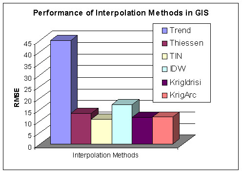
Figure 3.Comparison of Root Mean Square Errors
Similarly, the mean absolute error values indicated that TIN (Figure 4.) performed better than any other interpolation method within the GIS environment on this data. On average the TIN interpolation error was 7.38 ft based on a random sample of forty. The ordinary Kriging results from Idrisi and Arc-Info yielded the mean absolute error 8.57 and 8.53 ft. Interpolation from Thiessen polygons indicated the mean absolute error of 9.2 ft and IDW 12.6 ft. The trend surface interpolation error was on average 34.8 feet, the highest error from all interpolation methods. The mean absolute error values become more meaningful if they are compared with the variance of errors. The interpolation using TIN, again, indicated the smallest variance of errors and hence showed the least uncertainty in predicting the values in an unsampled location. The error variance in Kriging also indicated values close to TIN. The ANOVA test statistics were used to compare errors from all six interpolation methods i.e. the zero hypothesis  was tested to determine whether the mean absolute error values from the six interpolation methods were significantly different. As the F-value of the test and associated p-value (0.001) indicated, the zero hypothesis was rejected in favor of the alternative hypothesis, i.e. not all interpolation methods performed equally well. The Tukey grouping differentiated between errors from the trend analysis and the rest of the interpolation methods at alpha level 0.05. This breakdown did not change until the alpha level was 0.6. Then the Tukey Test distinguished three groups: a) trend surface analysis (highest error producing interpolations) b) IDW (mediate error producing interpolation) and c) TIN, Kriging and Thiessen polygon (the lowest error producing interpolation methods in GIS).
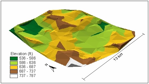
Figure 4.Piloncillo Surface from TIN Interpolation
Spatial analysis is often affected by the large errors. In order to determine the possible causes for extremely large interpolation errors, spatial distribution of the five largest mean absolute errors was studied in relationship to the slope values and general trend of the surface. As the analysis indicated in some cases the large interpolation errors tended to be distributed within the area of the large original values. However, the plot of observed (original) values and errors from TIN interpolation (Figure 5.) did not indicate this relationship. On the contrary, the large errors tend to be associated with the smaller observed values and the errors incline to decrease with large observed values. This might indicate a bias and suggests possible transformation of original data before the interpolation method is being applied. The large errors from the trend surface analysis indicated a strong relationship with high-observed values, whereas TIN showed no relationship of errors with the highest surface. In contrast, IDW errors indicated a relationship with high values in the original data. Kriging, similarly to the TIN and Thiessen polygon, did not indicate a bias with high-observed values. Therefore, each interpolation method responded differently to the original data set.
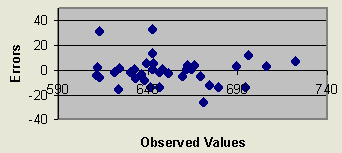
Figure 5.Spread of Errors from TIN Interpolation
CONCLUSION
The current research and industrial projects in GIS require higher standards for the accuracy of spatial data. Interpolation is one of the frequently used methods to transform field data, especially the point samples into a continuous form such as grid or raster data formats. There are several interpolation methods frequently used in GIS. In this paper the performance of six methods was evaluated based on the magnitude and distribution of errors. As the statistical analysis indicated, Kriging, IDW, Thiessen polygons and TIN performed almost on the same level, however, TIN appeared to be a leading method in predicting the values in an unsampled location on a more uniform, less varied data set (flat surface). It produced results with the smallest mean absolute error, smallest variance of error, the highest correlation coefficient between the predicted and observed values (Figure 6.) and the smallest correlation between the errors and observed values and is recommended by this analysis to GIS practitioners as a simple and efficient procedure to interpolate data and generate a map for pratical applications.
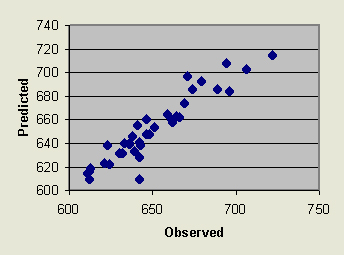
Figure 6.Observed vs. Predicted Values from TIN Interpolation
ACKNOWLEDGMENT
This project was supported by the College of Forestry at the Stephen F. Austin University.
REFERENCES
- Bancroft, B.A., and G.R. Hobbs. 1986. Distribution of Kriging Error and
Stationarity of the Variogram in a Coal Property. Mathematical Geology
8(7):635-651.
- Burrough, P.A., and R.A. McDonnell. 1998. Principles of Geographical
Information Systems. New York: Oxford University Press.
- Clark Labs. 2000. IDRISI32 I32.01 software. Clark University, MA.
- Esri. Environmental Science Research Institute, Inc. 1999. Arc/Info
8.0.1 software.
- Esri. Environmental Science Research Institute, Inc. 1999. ArcView 3.2
software.
- Goodchild, M., F. Guoqing, and Y. Shiren. 1992. Development and Test of an
Error Model for Categorical Data. International Journal of Geographical
Information Systems 6(2):87-104.
- Heuvelink, G.B.M., and P.A. Burrough. 1989. Propagation of Errors in
Spatial Modeling with GIS. International Journal of Geographical
Information Systems 3(4):303-322.
- Lam, N.S. 1983. Spatial Interpolation Method: A Review. American Cartographer 10:129-220.
- Mandel, J. 1984. The Statistical Analysis of Experimantal Data. New
York: Dover Publications.
- Siska, P. P., and I. K. Hung. 2000. Data Quality on Applied Spatial
Analysis. In: Papers and Proceedings of the Applied Geography
Conferences, Vol. 23. ed. F. A. Schoolmaster, 199-205.
- Siska, P.P. and R.C. Maggio. 1997. The Role of Relief Dissectivity in
Distribution of Kriging Errors from Digital Elevation Modeling. In: Papers
and Proceedings of the Applied Geography Conferences, Vol. 20, ed. F.A.
Schoolmaster, 186-194.
- Taylor, J. R. 1997. An Introduction to Error Analysis. 2nd ed.
Sausalito, CA: University Science Books.
AUTHORS
1)Peter P. Siska and 2)I-Kuai Hung
1)Assistant professor
2)Graduate student
College of Forestry
Stephen F. Austin University
Nacogdoches, TX 75962-6109
Phone: 936-468-1347 Fax: 936-468-2489
Email:siska@sfasu.edu