This paper presents the design and application of a simplified GIS-based hydrology model capable of ingesting NEXRAD radar rainfall. The distributed model was designed as an educational tool for providing a hands-on hydrologic modeling experience to undergraduate environmental engineering majors at MIT. A simplified approach was taken to watershed modeling in order to take advantage of the existing spatial analysis function within ArcView GIS and its Spatial Analyst and Hydrologic Modeling Extensions. The model couples a runoff generation subcomponent based on the Soil Conservation Service (SCS) approach and a DEM-based Travel Time routing method. In addition to data analysis and GIS model setup, aspects of model calibration and evaluation were considered during the teaching exercise. The model was applied to two river basin (Peacheater Creek Basin near Eldon, OK and Squannacook River Basin near West Groton, MA) for two storm events. The Squannacook case study consisted of a significant flooding event in June 1998, while the Peacheater creek storm event produced high-flow conditions during January 1998. Telemetered stream gauge data from the USGS was used to calibrate and validate the model response to the input NEXRAD rainfall fields. The modeling exercise was encapsulated within ArcView GIS and aided through model description procedures available at http://web.mit.edu/1.070/www/GISlab.html.
Heavy and/or persistent rainfall over a watershed can lead to serious flooding events that are the most devastating weather related hazard in the United States (NRC, 1996). The impact of flooding to human civilizations is a topic as old as recorded history, as evidence by Egyptian stage measurements (i.e. Eltahir and Wang, 2000). In modern times, civil engineers specializing in hydraulics and hydrology have been responsible in our society for studying the causes and attempting to predict the onset of flooding events prior to their occurrence. Our ability to predict flooding events has significantly increased due to the availability of new data sources and the proliferation of hydrologic models that capture the essential processes governing water flow on the land portion of the Earth. New data sources include the observation and estimation of precipitation from remote sensors including land-based radars as well as space-based radiometers, imagers and radars. Improved description of the land surface characteristics on the Earth, including high resolution topography, soil and vegetation, have also been incorporated into advanced models that attempt to predict the spatial distribution of hydrologic response.
Along with the availability of new data sources and hydrologic models, the use of Geographic Information Systems (GIS) in hydrologic prediction has been an important advancement in the last decade (ASCE, 1999). The data management, analysis and visualization capabilities inherent in a GIS have greatly simplified the analysis of digital elevation models (DEMs), soils, land use, vegetation and geological data, as well as the derivation of the hydrologic network. Today, most advanced hydrologic models use GIS as a data preprocessor tool in a loosely-coupled sense (Miles and Ho, 1999). While this is valuable, the integration of a GIS with a hydrologic model can be performed under conditions of tighter coupling. By relating watershed and hydrologic data to a map-centered model grid, a tightly coupled GIS hydrological model can update model and data features simultaneously. In this approach, GIS technology can be used for data management, storage and visualization, in addition to model creation, execution and calibration. As one example of this approach, Ye (1996) presented the development of a subsurface and surface hydrologic model entirely within ArcView GIS.Recognizing the need for simplified watershed models within a GIS environment, this study focused on creating an infiltration-excess runoff model entirely within ArcView GIS to be used as an educational tool for undergraduate environmental engineering majors at the Massachusetts Institute of Technology (MIT). A collection of Avenue scripts forms the basis for the raster-based model and uses the capabilities of the Spatial Analyst and the Hydrologic Modeling Extensions. ArcView GIS provides a common interface for model preprocessing of watershed and hydrometeorological data, model setup and execution as well as postprocessing of model output, including runoff maps and the stream hydrograph. An educational exercise was designed around the ArcView GIS Hydrologic Model for teaching students about hydrology in general and watershed modeling, calibration and validation in particular. The exercise was developed around two particular case studies: a significant flooding event in the Squannacook River Basin in Massachusetts and a high streamflow event in the Peacheater Creek Basin in Oklahoma. Extensive rainfall and watershed data sets were available for both case studies and used to drive the raster-based, distributed hydrologic model. Model calibration and validation were performed by comparing the simulated streamflow with in-situ measurements from the USGS stream gauge network.
Distributed hydrologic models rely on accurate representations of the watershed topography, soil and vegetation properties. Topographic representation through Digital Elevation Models (DEMs) has increased our capability of modeling the surface and subsurface hydrologic processes that govern the rainfall-runoff conversion. High resolution DEMs are readily available from the USGS at various spatial resolutions. For the purposes of this study, the 7.5 minute DEM product from the USGS (30 meters ground resolution) were obtained for the two watersheds of interest. We retain the high resolution despite the drawbacks in computational burden for the grid operations in ArcView since the topographic representation is a driving component of the spatially-varied watershed response to the radar rainfall data. Aggregation of the high resolution DEM data have been shown to introduce significant artifacts in the computation of hydrologic and geomorphologic basin properties (i.e. Walker and Willgoose, 1999). Within the ArcView-based model, the topographic data is used to derive the stream network and the hydrologic distance from each grid cell to the watershed outlet, an important property for the runoff routing scheme.
In addition to the topography, soil and land use properties are utilized in the ArcView GIS Hydrology Model to specify the land surface characteristics that determine the partitioning of incident rainfall into infiltration and runoff. The surface soil texture is typically used to determine the soil hydraulic properties and thus the capacity of the soil to absorb water through pedotransfer functions (i.e. Rawls and Brakiensek, 1985). The Natural Resources Conservation Service (NRCS) has produced digitized soil maps for the entire United States in the form of two products, the STATSGO and the SSURGO databases. In this study, we utilize the county survey-based STATSGO data which is a generalized representation of the pedological properties for the two basins of interest. For the land use/land cover maps, various products obtained from satellite imagery and local field surveys are readily available. In particular, a popular data source is the LULC database available from the EROS Data Center. The digitized land use maps are obtained by reclassifying satellite AVHRR images using a cataloging system produced by Anderson et. al (1976). Both the soil texture and the land use characteristics for each grid cell are used for the derivation of the curve number parameter (CN). This parameter is used in the model as a rainfall partitioning coefficient and varies according to soil type, land use class and antecedent moisture conditions.
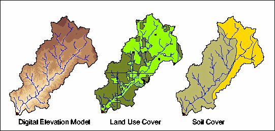
The Peacheater Creek Basin is a small subbasin of the Arkansas-Red River watershed, located in the northeastern corner of Oklahoma and approximately 64 square kilometers in total area. The watershed DEM reveals an extensive valley bordering the principal river and a distinct variability in valley density in the landscape. The elevation difference within the watershed is approximately 185 meters over a nominal watershed length scale of 13 kilometers implying a basin-averaged slope of 0.014 m/m. The vertical accuracy of the Peacheater Creek Basin DEM is approximately 1 meter. The DEM was hydrologically corrected by removing pits or sinks, thus ensuring a continuous water flow over the watershed. DEM processing was performed within ArcView GIS using the Spatial Analyst extension. Deriving the stream network in this example is composed of various steps including: (1) defining the cell slopes, (2) defining the flow directions, and (3) calculating the flow accumulations. With a threshold area placed on the definition of a stream, the stream network was derived and compared to the mapped blue-line vectors on the USGS Quad Sheets. Figure 1 demonstrates the Peacheater Creek DEM and stream network along with the soil and land use properties derived from the described data sources. Note that the watershed area is characterized by agricultural and forest lands with only minor urban features. The predominant surface soil type is silt loam in the region.
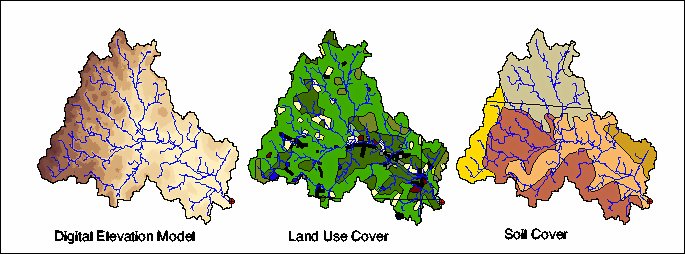
The Squannacook River basin drains into the Merrimack River in Eastern Massachusetts via a confluence with the Nashua River. Approximately 171 square kilometers in size, the drainage basin is a highly developed, urban watershed, including numerous water reservoirs and dams. The Digital Elevation Model reveals a west to east topographic gradient and a broad valley near the catchment outlet. The elevation range in the basin is from 807 to 5,783 meters with a stated accuracy of 2 meters in the vertical for the 7.5 minute DEM. The DEM has been hydrologically corrected by removing pits or sinks for water flow over the landscape. After this procedure, the stream network has been computed using local slope and direction information. Overlain on the DEM, the stream network reveals the importance of topography on stream channel formation. Figure 2 demonstrates the Squannacook River DEM and derived stream network, along with the the soil and land use properties for the watershed. As compared with the Peacheater Creek, this watershed is highly urbanized. Interspersed with the urban areas are the deciduous forests characteristic of New England. The soil types within the watershed are more diverse than in the agricultural watershed in Oklahoma.
The United States has invested significant resources in installing and operating a nationwide network of weather radars for the purpose of measuring precipitation in forms of rain and snow (Whiton et al, 1998). Since 1993, the NEXRAD (Next Generation Radar) system has been operational in many parts of the US, contributing significantly to weather forecasting and to the public dissemination of weather data. Today, the coverage of the NEXRAD radars for rainfall estimation is unparalleled throughout the world. For this study, we used the Stage III NEXRAD product available from the National Weather Service (NWS), as hourly values over an approximately 4 km by 4 km grid. It consists of the radar rainfall rate (in cm/hr) obtained after significant processing has been done to the data, including corrections to the reflectivity estimates and the conversion to a rainfall value based on an empirical Z-R relationship. Note that the radar itself does not measure rainfall rate, but rather the reflectivity of the rain droplets to a doppler radar pulse operating in volume scanning mode. The conversion from the reflectivity measurement to the hydrologic variable of interest is inherently imperfect. To alleviate this, the measurements from overlapping radars are combined and the results compared to rain gauge estimates over the region of interest (Fulton et. al, 1998).
The availability of the remotely-sensed precipitation estimate from NEXRAD has created significant opportunities in the ability of hydrologists to model the watershed response to rainfall. The driving reason for utilizing NEXRAD data in distributed hydrologic models are the spatial coverage and variability offered by the radar rainfall maps. Young et. al (2000) have recently tested the NEXRAD rainfall products for use in hydrologic forecasting models and various researchers have used NEXRAD data for predicting flood and flash flooding events (i.e. Warner et. al, 2000). In this study, we utilize the spatially-distributed rainfall maps obtained from the Stage III product to drive the watershed response in two basins of diverse climate, topographic and geologic characteristics for two significant streamflow events. The raster-based, distributed hydrologic model captures the spatial distribution and variability of the incident rainfall and integrates the input into a time-varying prediction of river flow at the basin outlet.
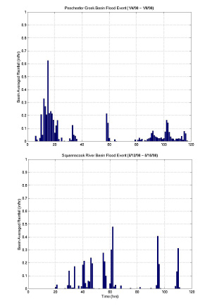
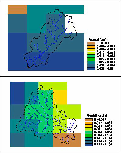
The Stage III NEXRAD data is obtained from the NWS as hourly raster grids organized by River Forecasting Center (RFC). For the Peacheater Creek basin study, the data from the Arkansas-Red River Forecasting Center (ABRFC) was used, while the Squannacook River model was driven with data from the Northeast River Forecasting Center (NRFC). The gridded data products were available in polar, stereographic projection at a resolution of approximately 4 km by 4 km. An ARC/INFO AML script was developed to process the Stage III data for input into the hydrologic model (Rybarczyk, 2000). The main steps in the processing consisted of: (1) projection onto a local UTM coordinate system (2) clipping with a bounding box surrounding the watershed of interest and (3) unit conversion. Time series plots of the average basin rainfall depth are shown in Figure 3 for the two events considered. The basin average hyetographs, however, do not portray the spatial variability in the incident rainfall over the watersheds as shown in Figure 4 for two particular time periods.
The United States Geological Survey (USGS) has installed, maintains and archives data from a nationwide network of stream flow gauges. The telemetered gauges measure the water depth at a particular river reach via the use of a pressure transducer or a bubble-pressure gauge. The river stage is converted into a discharge by knowing the precise relationship between the two, the so-called stage discharge relationship. In theory, if the cross sectional area at the reach is known from survey measurements, then a unique relationship between the stage and discharge exists. The USGS routinely measures the cross section at the stream gauges and converts the measured water depth to a discharge, which it then disseminates to the general public and to local governments. Real-time data access is now available for streamflow measurement through the USGS Real-Time Water Data Internet site (http://water.usgs.gov/realtime.html).
The Peacheater Creek and Squannacook River watersheds considered in this study both have stream gauges located at the watershed outlet and an established rating curve to determine the discharge at 15 minute intervals. The stream gauges correspond to the derived stream network outlet from the DEM analysis, as shown in Figure 1 and 2. The available data from the USGS is an hourly accumulation corrected for possible data errors. Two particular storm events have been chosen from the streamflow records for the two gauges: January 4 - 13, 1998 for the Peacheater Creek Case Study and June 12 - 22, 1998 for the Squannacook River Case Study. Figure 5 and Figure 6 demonstrate the streamflow hydrographs observed at the two gauging stations for the two hydrologic events under consideration.
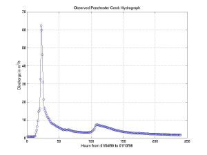
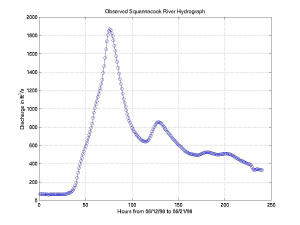
The winter storm event in the Peacheater Creek basin is a typical rainfall event occurring as a result of the passage of a frontal storm over the area. Neither the discharge measurement nor the rainfall amounts measured by NEXRAD radars and raingauges indicate that this storm was hydrologically significant. Nevertheless, it produced a greater than average runoff response within a short time period, as compared to the long-term flow record. The summer storm event over the Squannacook River basin was an atypical precipitation event due to an intense, slow-moving frontal storm in the New England region. This storm event was hydrologically significant due to its heavy rains in early summer (USGS, 1998). Although not the hardest hit by the rainfall, the Squannacook River Basin experienced a discharge with a recurrence interval of 3 years. Other streamflow gauges closer to Boston, such as the Aberjona River, experienced a flood with a 50-year recurrence interval (USGS, 1998).
There are a number of hydrologic models in existence today. These differ mostly in the hydrologic variables of concern and in the space-time region of model application. Watershed models tend to concentrate on the catchment as the basic hydrologic unit since this entity serves as a hydrologic control volume (Bras, 1990). As mentioned previously, the model developed in this study was applied to two mid-sized watershed (areas from 10-1000 square kilometers) that differ significantly in their climatic, topographic and geologic regimes. The model applications concentrated on storm event-based modeling, that is modeling a single high flow event for each basin. In addition, the model discretizes the watershed domain into a raster grid and models the hydrologic processes in the computational elements using conceptual approaches to runoff generation and runoff routing. In summary, the ArcView-based Hydrologic Model developed and applied for this teaching exercise can be classified as:
We have implemented two methods within the ArcView GIS Hydrologic Model to account for the generation of runoff from the NEXRAD rainfall input and the runoff routing along the stream network. One is an empirical equation that accounts for the conversion of rainfall to runoff depending on the land surface condition (in this case, a static quantity) and is called the Soil Conservation Service Method for Runoff Production. The second is a simplified hydrologic routing scheme based on the travel distance from the watershed cells to the outlet and an assumed hillslope and channel velocity (in this case, also static quantities). We refer to it here as the Travel Time Method. Together, these two methods provide a simplified approach to hydrologic modeling that only requires the calibration of three parameters and uses the full information available from the spatially distributed topography and radar rainfall input. Of the three parameters, one accounts for the rainfall-runoff partitioning (CN) and the other two for the overland and channel flow velocities (Vo and Vc). Description of these two methods follow.
The SCS method is widely used for estimating floods on small to medium-sized ungauged catchments in the United States (Bras, 1990). The method is an empirical approach to estimating infiltration within a watershed based on the characteristics of the land surface. The excess rainfall is available for runoff routing over the watershed surface and into the stream network. The following equation is the basis of the SCS method (Equation 1):
where Q = runoff depth (in), P = precipitation (in), Ia is initial abstraction (in) and S is the potential maximum retention after runoff begins (in). S is estimated from the land surface properties using an empirical relationship to CN, the curve number (Maidment et. al, 1993). The curve number is a coefficient estimated from the land surface characteristics (soil property, land use, hydrologic conditions and hydrologic group). Several tables are available to estimate it from the watershed data given for each basin. The relationship between S and CN is (Equation 2):
The initial abstraction, Ia, has been empirically related to the retention S as Ia = 0.2S. This parameterization allows us to reformulate Equation 1 in terms of the curve number (CN) (Equation 3):

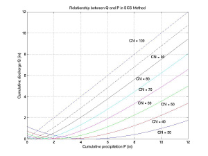
We could use Equation 3 to determine Q in inches for each hour of rainfall P given the knowledge of CN for each watershed grid cell. Taking a closer look at the form of Equation 3, however, reveals some of the limitations of this approach. If we plot Q versus P over a series of P values and for the family of CN curves, we observe a peculiar behavior for rainfall values less than a few inches, as shown in Figure 7. The SCS Equation predicts decreasing runoff for increasing rainfall for low values of P. This situation rarely occurs when the SCS method is used to model the cumulative runoff given a cumulative storm precipitation since the accumulated amount typically exceeds a few inches in value. However, on the hourly time scale used with NEXRAD rainfall data, precipitation is usually less than a few inches per time step and applying the SCS method in Equation 3 is not appropriate.
In lieu of this, this study adapted the SCS method by using a simpler model for runoff generation, one that states that runoff is a constant proportion of rainfall. This proportion is dictated by the condition of the land surface, mainly its hydrologic state and the soil infiltration properties, as parameterized by the curve number. Thus, the model generates runoff at each watershed pixel using Equation 4, where the curve number (CN as a percentage) is used to describe the rainfall and runoff conversion (Equation 4):
The watershed data gathered for the Peacheater Creek and the Squannacook River catchments was used to obtain the curve number of each individual watershed cell. The raster grid is discretized into 30 meter by 30 meter cells, according to the spatial resolution of the 7.5 minute DEMs. Each cell is assigned a value for soil texture and land use based on the thematic layers shown in Figures 1 and 2. From these characteristics, the curve number CN for each watershed pixel can be determined by using a reclassification table (e.g. Maidment et. al, 1993). The use of the reclassification table requires knowledge of the soil hydrologic group and the land cover type. The soil hydrologic group is determined from the textural information and the drainage characteristics available from the STATSGO database. The hydrologic groups are classified as:
A reclassification table for the two watersheds was derived from the soil property and land coverage data as shown in this Curve Number Table. An initial curve number grid was derived prior to the teaching exercise and given to students as a basis for Model Calibration. Variations in the curve number grid were an essential means for students to improve model simulations of streamflow relative to the observed values. An automated parameter updating scheme was created within ArcView GIS that allowed students to change the curve number values for each soil hydrologic group/land use class combination.
The SCS Method was used to estimate the runoff depth Q at each grid cell for each hourly time interval given the NEXRAD rainfall data. In order to compare the model results to the observed hydrograph at the watershed outlet, a simplified method for routing the runoff produced at all watershed grid cell was developed. The routing scheme is based on the travel distance or time for every grid cell to the outlet along the hydrologic pathways derived from the DEM of the watershed. We only consider overland and channel flow without taking into account the mechanisms of runoff generation occurring in the unsaturated and saturated zones. By choosing the DEM flow pathways, the runoff routing mesh is fixed by the topographic structure over all time. The travel distance is obtained readily by using the Hydrologic Extensions in ArcView GIS and a routine that traces a water parcel from each grid cell to the outlet. Each cell has a different pathway to the outlet, part of which occurs over an overland portion and the other part within a stream channel. By assigning a velocity for the overland flow portion Vo and a velocity for the channel portion Vc, the total time of travel to the outlet for each volume of water produced at each pixel at each hourly interval can be computed. Assuming spatially-uniform and time-invariant velocities is not an unreasonable assumption in simplified watershed models of this nature (Wyss et. al, 1990). It does, however, introduce significant simplifications to the hydrologic routing scheme by reducing the calibration problem to two parameters governing the flow velocity in hillslopes and in channelized regions.
Having developed the Travel Time Method for hydrologic routing, a means for estimating the overland flow and channel flow velocities is required. In addition to the curve number grid, these two parameters serve as the basis for the calibration of the ArcView GIS Hydrology Model during the model application case studies. As expected from the Manning equation for discharge, the hillslope overland velocity should be smaller than the channel velocity because of the increased surface roughness and decreased water depth in unchannelized flow. A set of initial guesses were provided to the students, Vo = 0.1 m/s and Vc = 1 m/s, for preliminary model runs. Variations in the two velocity variables were part of the calibration exercise the students were asked to perform with the purpose of matching the simulated runoff with the observed discharge measured by the USGS. An automated parameter updating procedure was implemented in ArcView GIS to facilitate the calibration process.
The ArcView GIS Hydrology Model implemented in this study simulates the outlet hydrograph for each basin given the incident rainfall data derived from the NEXRAD radars. A hydrograph is simple a curve representing the discharge at a point in the stream network for each time period. It can also be thought as a concentration of water curve in the river. Computationally, it is derived by knowing the runoff at each grid cell at each time period and knowing the amount of time it will take that "package" of water to travel to the outlet. At the outlet, the model sums all the "packages" of water arriving from the discrete points in the catchment for each time period. At first, only a small number will arrive (those closest to the basin). As time progresses, the hydrograph peaks at some value (peak discharge) at a some time (time to peak). In the most strict mathematical sense, the computation of a hydrograph is equivalent to computing the convolution integral for the system (Bras, 1990).
The shape of the hydrograph is affected significantly by the parameter values chosen for runoff production and hydrologic routing. In this model, the specification of the curve number grid determines the amount of runoff produced for a particular rainfall amount. Thus, the total runoff volume in the hydrograph changes when parameter adjustments are made to the curve number field, either in a uniform fashion or for each soil hydrologic group/land use combination. In general, changes to the velocity variables result in variations of the hydrograph timing as measured by the time to peak, for example. Calibration of the velocity variables should not affect the simulated runoff volume, although the same cannot be said about changes in the curve number field which do have an impact on the time to peak as well. Both sets of parameters can be adjusted in a systematic fashion by comparing the volume of runoff and time to peak for both the simulated and observed flows.
Our principal goal was to allow the students to run and calibrate the model without learning the details of GIS, but at the same time not making the use of a GIS completely transparent. The model is written entirely as a set of Avenue scripts and packaged as an Arcview project (see Figure 9). It could have been packaged as an extension but that may have added the complication of having students add an extension as their first GIS task. We provided the base data, which includes all the rainfall grids, soils data, Digital Elevation Models (DEM) and slope information for the two case studies. All computer work was accomplished on Athena, MIT's distributed computing UNIX environment. The required data was made available over Athena's file system, AFS, so that students could work on the project during the lab session in one of MIT's electronic classrooms, and outside of the lab session in any of the Athena clusters on campus.
Students were instructed to copy the Arcview project entitled "runoff.apr" into their home directories (see Figure 9). Upon opening the Arcview project, students selected their modeling basin based upon the two modeling scenarios offered. Once selected, the Digital Elevation Model was added automatically to the Runoff View. From the Digital Elevation Model, the participants created the Flow Directions and Flow Accumulations grids using tools available in the Hydrologic Modeling extension. The Flow Accumulations grid was particularly important in computing the distance from each cell to the outlet along the steepest path of flow. In addition to manipulating the DEM, the students were provided with a Curve Number shapefile that described the conditions of the land surface (soil hydraulic properties and land use). The Curve Number shapefile was automatically converted into a grid for calculation purposes, rather than using the Grid->Shapefile function. The Curve Number Grid determines the amount of runoff produced at each grid cell and is thus an important calibration parameter in the two modeling case studies. Figure 8 shows a screenshot of the Curve Number Grid within the ArcView project.
The next task required in the Modeling Process was for students create a Time Grid using an automated procedure developed within Avenue. The Time Grid specifies the interval of time from each watershed point to the outlet based upon the distance of travel and two velocities (overland and stream flow) set by the user in a dialog box. For purposes of the educational exercise, the assignment of two constant parameters describing the velocity of surface flow was deemed appropriate. A more complex model, with flow velocities based on slope, roughness, watershed area at each grid cell, is quite possible and could easily be executed within the existing Avenue scripts. Subsequent to developing the Time Grid, the students converted it into a set of separate Time Slice Grids. The Time Slice Grids classify watershed area according to the travel time to the outlet in units of hours, as specified by the observed hydrograph. In addition to being used in the hydrograph computations, the Time Slice Grids were useful for observing how changes in the calibration process affect the model output (see Figure 9). In the last step, the students ran the hydrology model by forcing it with NEXRAD radar rainfall data stored in a remote AFS locker. The rainfall data were stored in grids which the same extent and cell size as the Curve Number Grids and the Time Slices Grids.
The model calculations were straightforward and based on the traditional computation of a watershed hydrograph. For each time slice, and for each hour of rainfall, the rainfall is multiplied by the Curve Number grid and divided by 100, as expressed in Equation 4. This yields the runoff amount for each individual grid cell in the watershed. The current time slice and the runoff grids are multiplied by each other yielding the volume of runoff per hour for each time slice region. The resulting volume of runoff represents the amount of water that reaches the outlet during one hour from that region. Each of the time slice grids are ordered: regions within 1 hour travel time to the outlet, regions within 2 hours travel time to the outlet, regions within N hours travel time to the outlet. The volumes for each of these are loaded into a table for the first hour of rainfall. For the second hour of rainfall, the volume grid representing regions within 1 hour of the outlet is added to the second hour of runoff and so forth. All of the data was aggregated into the hydrograph output table which represents the streamflow passing through the outlet during and shortly after the storm. The students used the provided curve number grid and overland and stream flow velocities for the first run of the model. The output hydrograph table was stored as an Arcview Table and also exported into an ASCII text file for use within MATLAB. After comparing the uncalibrated results with the observations, the students were instructed to improve the model performance through a calibration procedure.
The calibration procedures were automated within ArcView with the use of dialogue boxes and direct manipulation of the shapefile tables. Figure 10 shows examples of the dialogue boxes created within the ArcView project for model calibration. This enabled the students to quickly assess the effect of parameter changes without incurring in time-consuming changes to the model. Calibration was performed using three parameters: the overland flow velocity, the stream flow velocity, and the runoff curve number grid. Changing the velocity parameters through a dialogue box leads to a different travel Time Grid, as well as a different number of Time Slice Grids. Changing the Curve Number Grid was performed using a Update Function which queried the user for two possible types of changes: based on individual changes to the soil-land use group or shifts for the entire set of curve number classifications. After making the appropriate calibration changes, the hydrology model was run again and the resulting modeled hydrograph is compared to the actual hydrograph. If large discrepancies still exist, additional changes to the velocities and curve number grids can be automatically made and the calibration process continued.
Model calibration is an exercise performed during any modeling task. It consists of finding the model parameters and combinations thereof that allow the simulation to perform well as compared to a calibration target using appropriate measures for fitness. For this distributed parameter model, the target or measure for model performance is the integrated system output, the streamflow hydrograph, after the runoff has been routed to the watershed outlet. Although this is not the only available measure for model performance, it is the most commonly used in hydrology and can give insight into the integrated watershed response. Nevertheless, utilizing hydrograph matching as our calibration criteria does not ensure that the interior hydrologic processes, such as runoff production, are properly modeled. In fact, the simplicity of the representation of most watershed models suggests that the calibration exercise results in a simulated response at the outlet that is more-or-less correct, but for the wrong reasons. This is a widely debated subject in the hydrological literature (e.g. Beven, 1993).
In this study, the calibration procedures formulated during the teaching exercise consisted of finding the most appropriate parameters for the SCS runoff production and the Travel Time hydrologic routing model components. The curve number for each landuse-soil hydrologic group was one set of model parameters used to calibrate the runoff production in the model, while the overland and channel flow velocities were the two parameters controlling the routing component. The goal of the calibration exercise was to match the time of the hydrograph peak and total runoff volume as compared to the observed streamflow at the USGS stream gauge. Each individual student was asked to perform his or her own calibration based on a preliminary model run provided using estimates for the two velocities and a curve number grid. The students were expected to explore the parameter space by any means they felt was appropriate having in mind how the variations of each parameter would impact the runoff volume, timing or both. The challenge for the students was then to obtain the best possible simulated result for one of the basins assigned to them. Comparisons among students with different case studies were designed to highlight the differences in the two hydrologic responses in the two distinct watersheds.
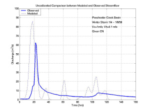
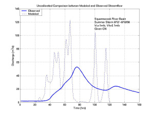
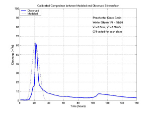
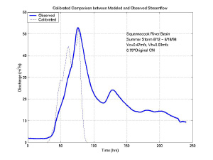
Uncalibrated model results given to the students for the two case studies in the Peacheater Creek and Squannacook River watersheds are shown in Figure 11 and Figure 12. Model performance without calibration is reasonable for the Peacheater Creek case study, but poor for the Squannacook River case study as compared to the observed hydrographs. For both cases, however, there is a need to modify the total runoff amount and the peak timing. After performing multiple calibration runs, the students submitted their best cases as part of the project assignment. These "best" results were pooled from the group of students and are shown in Figure 13 and Figure 14 for the two cases, respectively. It is apparent that the Peacheater Creek case study was modeled adequately using the ArcView GIS Hydrology Model developed in this study, while the Squannacook River case study, despite significant efforts, was not properly modeled to its fullest extent. The reasons behind this discrepancy have to do with the formulation of the modeled hydrologic processes and the characteristics of the watershed response to the NEXRAD rainfall patterns.
The model calibration exercises and the observed differences in the two case studies provided an opportunity to introduce students to various topics within the scope of modeling hydrologic processes. Issues concerning model parameterization and equifinality of the calibrated parameters were discussed in light of the different storm events and the varying characteristics of the two watersheds. As a final part of the teaching exercise, students were asked to answer the following questions related to hydrologic modeling as they experienced it in this exercise:
The design of the educational tool presented in this study was directed towards providing undergraduate environmental engineering majors at MIT with an opportunity to experiment, first-hand, with the set up and execution of a hydrologic model completely within a GIS environment. ArcView GIS provided a common interface for watershed and rainfall data manipulation, model parameter input and calibration, model execution and visualization of spatially-distributed results. The creation of the ArcView-based model allowed the teaching exercise to concentrate on the topic of interest, hydrologic modeling using NEXRAD data, without the unnecessary distractions that are customary in model setup, input and execution. In this sense, GIS served an important purpose of facilitating the introduction of students to the general topic of hydrologic modeling and its various steps.
In terms of the hydrologic model itself, despite the simplifying assumptions made in its construction, it performed reasonable well for one case study and poorly for another. The distinct behavior allowed for a comparison to be made about how the model represents hydrologic processes, an important insight for a newcomer to the field. The feedback from the student participants tended to emphasize what processes were not captured by the model and how it could be improved upon. This results directly from their understanding of the simplifying assumptions made during its development and their prior knowledge concerning the complexity of hydrologic processes in watersheds. For undergraduates to be introduced to the subject of hydrologic modeling to this extent and have first-hand experience in calibrating a simplified model is arguably an important contribution of this study to their education as environmental engineers.
This paper presented aspects of the design and application of a simplified GIS-based hydrology model for catchment scale rainfall/runoff modeling using NEXRAD data. The distributed model was used as an educational tool in the Department of Civil and Environmental Engineering at MIT for providing a hands-on hydrologic modeling experience to undergraduates. The implementation of the model entirely within ArcView using Avenue scripts along with the Spatial Analyst and Hydrologic extensions is an example of the integration of modeling capabilities within a GIS environment. The simplified hydrologic approach and the well-designed ArcView project facilitated the introduction of a complex subject matter to the undergraduates. Model performance stimulated inquisition into the hydrologic processes occurring in the two hydrologic events chosen as case studies. Experience using this model and the teaching exercise suggests that the integrated modeling approach is useful for educational purposes. A minor drawback to the approach, however, is the computational inefficiency of current GIS models for highly dynamic systems that require real-time processing, as suggested by Shutz (1996). Ingestion of NEXRAD data and hydrologic computations on the gridded watershed data on an hourly basis present quite a challenge for the ArcView platform. For basins with larger dimensions than those studied here, the model applications would have taken unacceptably long computational time for the teaching exercise.
American Society of Civil Engineers. 1996. GIS Modules and Distributed Models of the Watershed. ASCE. Reston, VA.
Anderson, J.R., Hardy, E.E., Roach J.T., and Witmer R.E. 1976. A Land Use and Land Cover Classification System for Use with Remote Sensor Data. U.S. Geological Survey Professional Paper 964, Reston, VA: U.S. Geological Survey.
Beven, K. 1993. Prophecy, reality and uncertainty in distributed hydrologic modeling. Advances in Water Resources. 16: 41-51.
Bras, R.L. 1990. Hydrology: An Introduction to Hydrologic Science. Addison-Wesley Publishing Company. Reading, MA.
Eltahir, E.A.B and Wang, G. 1999. Nilometers, El Nino and Climate Variability. Geophysical Research Letters. 26(4): 489-492.
Fulton, R.A., Breidenbach, J.P., Seo, D-J., Miller, D.A. and O'Bannon, T. 1998. The WSR-88D Rainfall Algorithm. Weather and Forecasting. 13: 377-395.
Maidment, D.R. 1993. Handbook of Hydrology. McGraw-Hill, Inc. New York.
Miles, S.B. and Ho, C.L. 1999. Applications and issues of GIS as Tool for Civil Engineering Modeling. Journal of Computing in Civil Engineering. 13(3): 144-152.
National Research Council. 1996. Toward a New National Weather Service: Assessment of Hydrologic and Hydrometeorological Operations and Services. National Academy Press. Washington, DC.
Rawls, W.J. and Brakensiek, D.L. 1985. Prediction of soil water properties for hydrologic modeling. Watershed Management in the Eighties. ASCE. 293-299.
Rybarczyk, S.M. 2000. Formulation and Testing of a Distributed Triangular Irregular Network Rainfall/Runoff Model. M.S. Thesis. Massachusetts Institute of Technology. Cambridge, MA.
Shultz, G.A. 1996. Remote sensing and GIS from the perspective of hydrological systems and process dynamics. HydroGIS 96: Applications of Geographic Informations Systems in Hydrology and Water Resources. Hovar, K. and Nachtnebel, H.P., ed. IAHS Publication no 235. IAHS Press. Wallingford, UK.
United States Geological Survey. 1998. The Flood of June 1998 in Massachusetts and Rhode Island. USGS Fact Sheet 110-98. Available online : http://ma.water.usgs.gov/floods/floods.htm.
Walker, J.P. and Willgoose, G.R. 1999. On the effect of digital elevation model accuracy on hydrology and geomorphology. Water Resources Research. 35(7): 2259-2268.
Whiton, R.C., Smith, P.L., Bigler, S.G., Wilk, K.E., and Harbuck, A.C. 1998. History of Operational Use of Weather Radar by U.S. Weather Services. Part II: Development of Operational Doppler Weather Radars. Weather and Forecasting. 13: 244-252.
Wyss, J., Williams, E.R. and Bras, R.L. 1990. Hydrologic modeling of New England River Basins using Radar Rainfall Data. Journal of Geophysical Research. 95(D3): 2143-2152.
Yates, D.N., Warner, T.T. and Leavesly, G.H. 2000. Prediction of a flash flood in complex terrain. Part II: A comparison of flood discharge simulations using rainfall input from radar, a dynamic model and an automated algorithm system. Journal of Applied Meteorology. 39: 815-825.
Ye, Z. 1996. Map-based Surface and Subsurface Flow Simulation Models: An Object-Oriented and GIS Approach. PhD. Dissertation. University of Texas, Austin. Austin, TX
Young, C.B., Bradley, A.A., Krajewski, W.F., Kruger, A. and Morrissey, M.L. 2000. Evaluating NEXRAD Multisensor Precipitation Estimates for Operational Hydrologic Forecasting. Journal of Hydrometeorology. 1: 241-254.
The authors would like to acknowledge the support received from the Ralph M. Parsons Laboratory and MIT Information Systems in conducting this study. In particular, the help of Steve Margulis and Prof. Dara Entekhabi in developing and conducting the course curriculum and Matt Van Horne and Liz Willey in preparing the calibrated storm hydrograph results are acknowledged.
Enrique R. Vivoni
Graduate Research Assistant, Ralph M. Parsons Laboratory
Massachusetts Institute of Technology, Cambridge, MA 02139
vivoni@mit.edu, http://web.mit.edu/vivoni/www
(617) 253-1969
Daniel D. Sheehan
GIS Specialist, MIT Information Systems
Massachusetts Institute of Technology, Cambridge, MA 02139
dsheehan@mit.edu
(617) 252-1475