Modeling Historical Exposures from Residential Proximity to Pesticide Applications

We developed a GIS-based model to assess historical pesticide exposure of residents living in Central California that will allow us to estimate study subjects’ exposure likelihood from residential proximity to pesticide applications. The model is based on two datasets: 1) pesticide use data from the California Pesticide Use Report (PUR) system from 1972 to the present, and 2) detailed California county land-use maps. Our model assumes that the likelihood for exposure from residential proximity to the use of a specific pesticide is based on: 1) the proportion of crop acres treated, 2) the application rate, and 3) the application frequency.

Background

Case reports and experimental and epidemiological research conducted over the past few decades suggest that chemicals used as pesticides may have an etiologic role in the neurodegenerative process leading to idiopathic Parkinson’s disease (PD). The finding that MPTP (1-methyl-4-phenyl-1,2,3,6-tetrahydropyridine), a neurotoxic byproduct of synthetic heroin, caused rapid and severe parkinsonian symptoms in humans, by specifically targeting the dopaminergic neurons in the substantia nigra, led many researchers to study chemicals and their possible involvement in the induction of PD (Betarbet et al., 2000).

Factors that have been shown to increase the risk of PD in epidemiologic studies include age, white race, genetic factors, rural living, well water use, farming, pesticides and other environmental and occupational toxins (Hubble et al., 1993). Also, some drugs, infections, tumors and cerebrovascular damage have been known to cause parkinsonian-like symptoms (Lang et al., 1998). It seems probable that there are many factors (genetic and environmental) involved that interact to result in PD.

Paraquat, a commonly used herbicide, has been studied because of its structural similarity to MPP+ (the toxic metabolite of MPTP). Dieldrin, an organochlorine pesticide, was found in increased concentrations in post-mortem brain samples in the brains of PD patients (Fleming et al., 1994). Rotenone, a “natural” herbicide commonly used by gardeners, caused parkinsonian symptoms in rats, including the typical Lewy body-like inclusions of PD (Thiffault et al., 2000). A variety of isoquinolones and beta-carbolines, used as pesticides, also exhibit similar toxic mechanisms to these pesticides (Jenner, 2001). In addition, concerns of biological interactions between various pesticides have arisen. For example, some carbamate fungicides have been observed to enhance the neurotoxicity of MPTP (Bochetta and Corsini, 1986). In a recent proportional mortality study, increased PD mortality was observed in rural California counties with high use of agricultural pesticides (Ritz and Yu, 2000). Since several herbicides resemble MPTP in chemical structure and pesticides are used heavily in rural areas, it is important to study their possible link with PD (Barbeau et al., 1987).

These findings contributed to the initiation of the Parkinson’s, Environment, and Genes (PEG) study, which is a population-based case-control study examining the role of gene-environment interactions in the etiology of PD. Over 5 years, we will be recruiting incident PD cases from three counties (Kern, Tulare, and Fresno) in the California Central Valley as well as population and sibling controls. While the induction of PD may occur over several decades, it will be important to assess historical exposures to pesticides from various pathways. As a result, we will conduct extensive interviews on residential and occupational use of specific pesticides. In addition to the historical exposures ascertained from subject recall, it will be necessary to ascertain potential exposures from other pathways, including residential proximity. With pesticide application data available from 1972 to the present from the California Department of Pesticide Regulation, we have developed a geographic exposure model to accomplish this task (Ritz et al., 2000). While other epidemiologic studies have been limited to small-scale estimates of exposure with a high potential for misclassification, we propose the incorporation of land-use information to increase the spatial resolution of the model. This paper will discuss the features of the model.

Data Sources: Pesticide Use Reports and Land Use Surveys

California has mandated the filing of PUR for applications of restricted-use pesticides since 1972 and all pesticides since 1990 (Department of Pesticide Regulation, 2000). Included in each detailed PUR is the name of the applied pesticide and pounds applied, the applied crop and acreage, the application method, and the date and location of the application to within a Public Land Survey (PLS) section with an area of approximately one square mile. We will be using the PUR data as the basis for modeling potential exposures from residential proximity to specific pesticides over several decades. Detailed residential histories will be collected from study participants along with information on residential and occupational use of pesticides. Below is an example of a report:

County: Kern

Location (County_Meridian_Township_Range_Section): 15M28S27E19

Application date: 2/23/1989

Commodity code: 2503 (Grapes)

Application Method: Ground

Treated: 424 acres

Product applied: 155 gallons

Chemical: 00459 (Parathion)

Percentage of active ingredient: 80%

Active Ingredient Pounds: 1,241

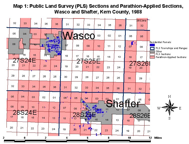
Despite the high level of detail in the PUR, the resolution of the data to only one PLS limits the ability to identify the most likely locations for a particular application. This is illustrated in Map 1 , where 36 sections (approximately 640 acres) make up one township-range (e.g., 27South25East) in the vicinity of Wasco and Shafter, northeast of Bakersfield, Kern County. The shaded squares indicate sections reporting any applications of parathion in 1988. We would only be certain that the application of a pesticide on a specific crop occurred somewhere inside the PLS section square, even if the crop only covered a small portion of the section.

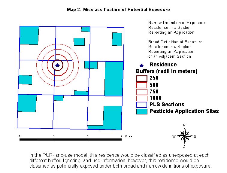
PUR data has been used to assess small-scale county- and local-level potential exposures to specific pesticides in various ecologic and individual-level epidemiologic studies. In previous studies using PUR data, exposures from residential proximity to pesticide applications have been defined as residence within a reported PLS section (narrow definition) or as residence within a section with a reported application or adjacent to another section with a reported application (broad definition) (Bell et al., 2001; Impact Assessment, Inc., California Department of Health Services Environmental Health Investigations Branch, 1998). Using PUR data with a spatial resolution of only one square mile, however, there may be substantial misclassification of broadly- or narrowly-defined exposure if the pesticide application actually occurred at a considerable distance from the residence. This method is insufficient for defining exposures at variable distances from pesticide applications, particularly when potential exposure can better be defined as residence at variable distances to reflect uncertainty in assessing exposure.

Map 2 illustrates misclassification of a residence’s broadly- and narrowly-defined potential exposure. Assuming that exposure occurs within a fixed radius from the residence, the likely area of pesticide application is a substantial distance away from the residence, although the residence would be classified as potentially exposed using either the broad or narrow definition.

To minimize misclassification of potential exposure, it will be necessary to increase the spatial scale of the model beyond one square mile. Without additional geographic information, however, we are unable to determine the specific location of the reported pesticide application within the PLS section and thus estimate potential exposure on a larger scale.The spatial resolution of the post-1990 PUR can be improved to specific locations within a PLS section by linking the data to site license information. Before 1990, however, site license information is not available.

As a result, we are using land-use maps to increase the spatial scale of pre-1990 PUR data. The California Department of Water Resources periodically performs countywide surveys of land use and crop cover (California Department of Water Resources, 1971). These large-scale (1:24,000, or 1 inch = 2000 feet) surveys are conducted every 7-10 years, and allow us to locate specific crops within each PLS section, and thus determine more precisely the location within a section where a specific reported pesticide application occurred. By restricting PUR to the likely sites of application within a PLS section, this land-use information can increase the specificity of assessments of potential exposure and thus minimize misclassification of potential exposure.

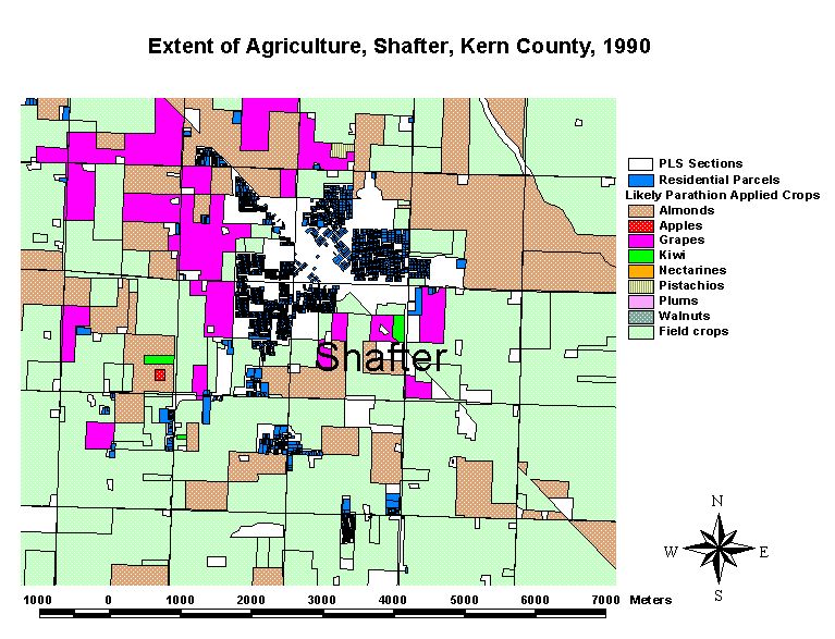
Seasonal rotations of field, truck, grain, and pasture crops as well as the 7-10 year period between surveys, however, will lead to uncertainty regarding what specific crop was planted in a specific location at a point in time. As a result, to acknowledge this uncertainty, we collapse these crops together into a class of field crops and assume that for a reported application of a pesticide on a specific field, truck, grain, or pasture crop in a section, all areas of these crops are equally likely sites of application (See Table 1). We are currently examining methods for increasing our certainty of seasonal crop locations by applying probability weights for crops with similar characteristics and crops that may be rotated with each other. Nevertheless, for orchard stands and vineyards (which may stand for several decades), their locations in the years preceding and following the surveys will not be substantially different from the locations indicated by the land-use survey. As a result, the exposure model will be much more specific for applications on orchard crops than on field crops.

Map 3 shows the extent of orchard and field crops around Wasco and Shafter. In this region, almonds and vineyards are the predominant orchard crops. The commodities making up the field crops are listed in Table 1.

Table 1. Field crops included in collapsed land-use classification

PUR/Land-Use Proximity Model and Comparison to PUR-only Proximity Models

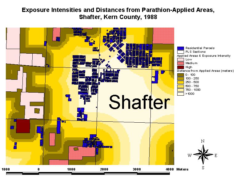
Identified by both the PUR and land-use information, the likely pesticide-application sites are mapped using ArcView GIS. To determine distances of subjects’ residences to the nearest application site, a distance surface is generated using Spatial Analyst. A residence would be potentially exposed if it was within a fixed distance from a likely application site and potentially unexposed if it was outside of that fixed distance. As a result, exposures can be much more flexibly defined for multiple analyses than the PUR-only model with only two options (broad and narrow) for defining exposure. Map 4 illustrates both the likely application sites and the distance surface. Residential parcels are also shown to demonstrate the proximity of the city of Shafter to the likely application sites.

Due to the extensive manpower required to digitize the maps from paper, it will be necessary to determine the impact the land-use data have on increasing the quality and minimizing the misclassification of the assessments of potential exposure.

Compared to our model utilizing two data sources, we expected the proximity model based only on PUR data to have poorer validity in assessing residential proximity to likely applications and the subsequent effect estimates (case-control odds ratios) to be biased toward the null, assuming nondifferential misclassification among cases and controls. We explored this issue by measuring the sensitivity and specificity of the narrow and broad exposure definitions compared to our “gold standard” of fixed distances from likely parathion application sites in 1988 in the surveyed (western) region of Kern County, excluding the non-agricultural urbanized areas of Bakersfield beyond 1000 meters of the city limit. Using residential parcels as the hypothetical residential addresses, we simulated 1000 random samples of 200 addresses (an approximation of the expected number of cases and controls from this portion of the county). We then measured the sensitivity (the proportion of residences within a specified distance of a likely application site that were classified as exposed in the broad or narrow PUR-only model) and specificity (the proportion of residences beyond a specified distance that was classified as unexposed in the PUR-only model) for each sample for fixed distances of 100, 250, 500, 750, and 1000 meters. From the median sensitivities and specificities, we calculated the observed biased odds ratios based on hypothetical “true” odds ratios of 1.5, 2.0, and 5.0 and case (diseased) exposure prevalences of 5, 10, and 15% to assess potential nondifferential misclassification (see Appendix). The results for broadly-defined (residence in a PLS section reporting a parathion application or an adjacent section) potential exposure are illustrated in Table 2.

Table 2: Sensitivity (SE), Specificity (SP), and Observed Odds Ratio (OR) and Exposure Prevalence Estimates Using the Broad Definition of Potential Exposure In Relation to Specified Distances from Likely Parathion Application Sites

As expected, the broad exposure definition had perfect sensitivity and increasing specificity with increasing distances. Observed exposure prevalences for cases and controls (not shown) were highly inflated and the observed odds ratios were attenuated toward the null. These results are what we expected, as the bias from nondifferential misclassification is more dependent on specificity than sensitivity. While this method will capture all potentially exposed cases at each specified distance, the poor specificity will drive the observed effect estimates toward the null.

The results for narrowly-defined (residence only in a PLS section reporting a parathion application) potential exposure are shown in Table 3.

Table 3: Sensitivity (SE), Specificity (SP), and Observed Odds Ratio (OR) and Exposure Prevalence Estimates Using the Narrow Definition of Potential Exposure In Relation to Specified Distances from Likely Parathion Application Sites

At each distance, the narrow exposure definition had near-perfect specificity and decreasing sensitivity at increasing distances. Observed case and control prevalences were inflated, but not as drastically as under the broad exposure definition. Observed odds ratios were biased toward the null, but the attenuation decreased for increased distances. At 1000 meters and perfect specificity, the observed odds ratios were very close to the “true” odds ratios. Although this result is specifically for parathion applications in 1988 in Kern County, it suggests that only for pesticides with substantial drift from the application site, exposure assessment using the narrowly-defined PUR-only model will not bias the effect estimates compared to the broad definition of exposure while at smaller distances, effect estimates based on either the broad and narrow exposure definitions will be biased toward the null. As a result, the greatest gain in validity from the land-use maps occurs when exposure is defined at smaller distances.

Quantification of Potential Exposure Intensity

In addition to measuring proximity to likely application sites, we would like to categorize the sites based on differences in the likelihood of exposure. To categorize potential exposure, three variables derived from the PUR and land-use data and assumed to be associated with an increased potential for exposure were combined in a weighted additive model. The following variables, along with their weights, are listed below:

1. Proportion of crop acres treated with the pesticide (50%).

2. Categorized application rate based on the recommended instructions specified on the pesticide labels as well as historical use (pounds of active ingredient applied/crop acres treated collapsed into categories of low, medium, and high rates; 40%).

3. Frequency of application (total number of months applied in a year; 10%).

The modeled estimates of potential exposure for pesticide-crop-section specific PUR are then mapped onto the likely sites of application. As in the proximity model described earlier, we can then determine residential proximity to likely sites, but with different intensity levels.

We are currently analyzing the sensitivity of this method to changes in the relative weights in the parameters as well as different categorizations of application rates. In addition, we are examining methods for incorporating application methods (aerial or ground), solvent type, and weather and wind data into the model. Although this current method is an oversimplification of categorizing levels of exposure, our preliminary findings suggest that the classifications do not significantly change with shifts in the variable weights.

Future Work

For a population sample in Kern County, we will be validating the PUR/land-use model by comparing results from residential histories against organochlorine levels detected in blood samples. We will test whether our exposure classification of each patient correlates well with his or her organochlorine blood levels as well as with exposure histories obtained from detailed telephone interviews.

In addition, we will attempt to determine drift potential for specific pesticides to determine the appropriate distances for categorizing potential exposure. Digitizing hundreds of large paper maps from several decades is an expensive time-consuming activity. As a result, we will continue to compare results between the PUR/land-use and PUR-only models to determine the usefulness of these maps (as well as their necessary labor) to the PEG study. To complement the model-based potential exposure assessments from residential proximity to applications, study participants will be interviewed about occupational, residential, and personal histories of pesticide use and exposure from other pathways, including mixing, handling, and applying specific pesticides.

To control for multiple comparisons involved in simultaneously analyzing numerous exposures, a hierarchical regression model will be utilized to facilitate the analysis of specific pesticides, classes of pesticides with similar toxicological properties, and combinations of pesticides with correlated use patterns (i.e., compounds applied to a specific crop).

Conclusion

Our model allows for flexible analysis of potential exposure from residential proximity to pesticide applications. With questionnaire data, we can obtain a more comprehensive assessment of historical exposure than if we had only used one tool. Our model, however, has several limitations, including uncertainty of the locations of specific field crops and the long periods of time between land-use surveys. In addition, it is based only on a few variables available from the PUR and land-use surveys and currently does not consider critical factors including weather, wind speed and direction, application method, and environmental fate of the pesticide following application. We are considering methods for incorporating these variables into the model. Nevertheless, our method, based on pesticide-use data unique to California and land-use surveys, is an improvement over previously developed methods for assessing historical pesticide exposures from residential proximity.

Appendix

Assuming non-differential misclassification and based on the “true” exposure prevalence in the cases (p₁), exposure prevalence in the controls (p₀), sensitivity (SE), and specificity (SP), the observed prevalences will be (Goldberg, 1975):

1)      for cases: p_o1 = p₁SE + (1-p₁)(1-SP)

2)for controls: p_o0 = p₀SE + (1-p₀)(1-SP).

The observed odds ratio will be:

OR = [p_o1/(1- p_o1)]/ [p_o0/(1- p_o0)].

References

Barbeau A, Roy M, Bernier G, Campanella G, Paris S. Ecogenetics of Parkinson’s disease: prevalence and environmental aspects in rural areas. Can J Neurol Sci 14:36-41 (1987).

Bell EM, Hertz-Picciotto I, Beaumont JJ. A case-control study of pesticides and fetal death due to congenital anomalies. Epidemiology 12:148-156 (2001).

Betarbet R, Sherer TB, MacKenzie G, Garcia-Osuna M, Panov AV, Greenamyre JT. Chronic systemic pesticide exposure reproduces features of Parkinson's disease. Nat Neurosci 3:1301-1306 (2000).

Bochetta A, Corsini GU. Parkinson’s disease and pesticides. Lancet (Nov 15):1163 (1986).

California Department of Water Resources. Land Use in California: An Index to Surveys Conducted by the California Department of Water Resources. 176. Sacramento: 1971.

Department of Pesticide Regulation, California Environmental Protection Agency. Pesticide Use Reporting: An Overview of California's Unique Full Reporting System. Sacramento: 2000.

Fleming L, Mann JB, Bean J, Briggle T, Sanchez-Ramos JR. Parkinson’s disease and brain levels of organochlorine pesticides. Annals of Neurology 36:100-103 (1994).

Goldberg JD. The effects of misclassification on the bias in the difference between two proportions and the relative odds in the fourfold table. J Am Statist Assoc 123:736-751 (1975).

Hubble JP, Cao T, Hassanein RS. Risk factors for Parkinson’s disease. Neurology 43:1693-1697 (1993).

Impact Assessment, Inc., California Department of Health Services Environmental Health Investigations Branch. Final Report: Analytical Procedures, Methodologies, and Field Protocols to Monitor and Determine Environmental Contaminants: Pesticide Use in California: U.S./Mexico Border Region. Oakland: 1998.

Jenner P. Parkinson’s disease, pesticides and mitochondrial dysfunction. Trends in Neuroscience 24(5):245-246 (2001).

Lang AE, Lozano AM. Parkinson’s disease: first of two parts. New Eng J Med 339:1044-1053 (1998).

Ritz, B, Rull, RP, Quach, T, and Krishnadasan, A. Modeling pesticide exposure in three Californian counties based on historical pesticide use reporting and proxy information. Epidemiology 11:S78 (2000).

Ritz B, Yu F. Parkinson’s Disease Mortality and Pesticide Exposure in California 1984-1994. Int Journal Epi 29:323-329 (2000).

Thiffault C, Langston JW, Di Monte DA. Increased striatal dopamine turnover following acute administration of rotenone to mice. Brain Research 885:283-288 (2000).