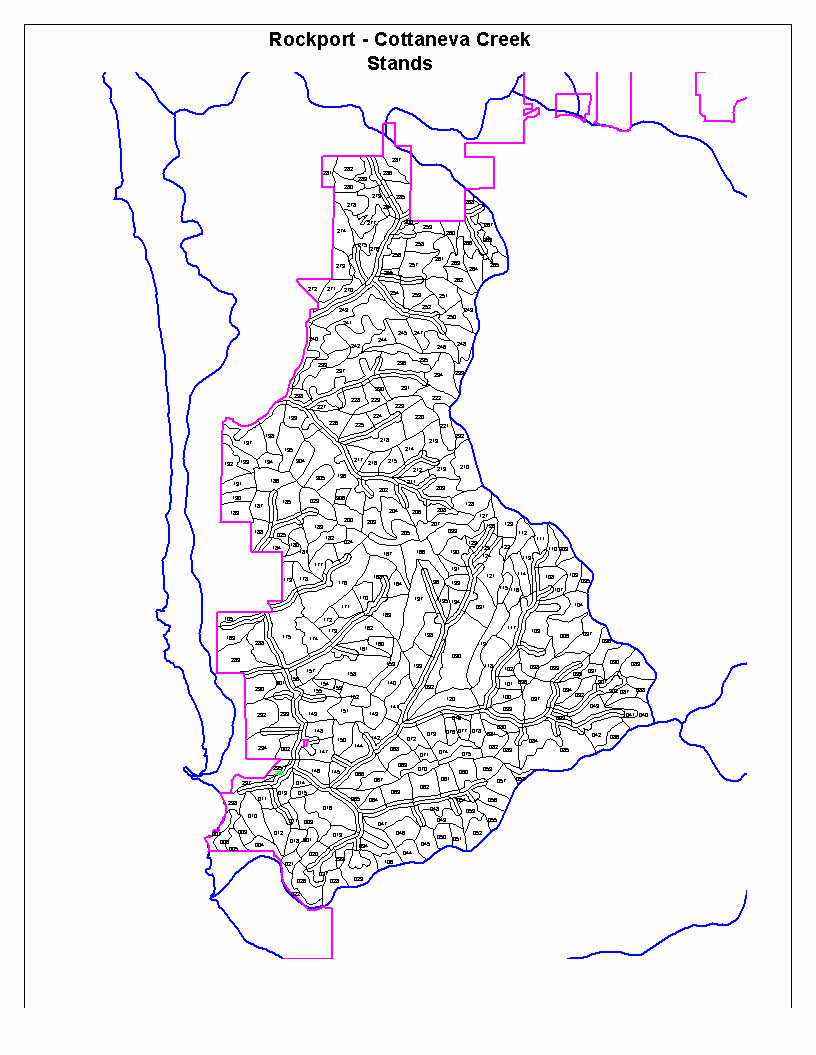
Figure 1. Stands digitized in ArcInfo serve as the base of linking all database and modeling activities to the GIS. Each stand has a unique identifier and is linked to MS Access database tables.
Forest landscape planning requires resource managers to consider many different factors. Successful management plans require multi-disciplinary input including resource specialists, managers, and the public. A ground-based approach to the development of strategic plans enables those who will implement the plans the ability to consider road networks, habitat conditions and sensitivities, and the spatial organization of management activities. ArcInfo is used to identify stands that are logical management units. Stands are the basic units that have tree lists and attributes in Microsoft Access. Stands are ‘grown’ and ‘harvested’ in 5-year periods in a Microsoft Visual Basic program. All outputs of the model can be mapped in ArcView for graphical presentation. 5-year plans are subsequently processed using ArcInfo to develop an optimal road use strategy to minimize erosion.
With timberland investment and ownership, resource management must consider both ecological sustainability and economic return, goals that seem to conflict. Successful strategic planning often depends on the degree to which those who will implement the plan are involved in the planning process. Input is necessary from foresters, biologists, hydrologist, geologist, and other specialists. Information must also be conveyed to the public. Previous efforts involved developing strategic plans based on remotely sensed data that was modeled to produce theoretically optimal management scenarios. The geographic area assessed for the strategic plans were not easily synchronized with management on the ground. Stakeholders had difficulty conceptualizing the process, determined the results unobtainable, and abandoned the plans.
Mendocino Redwood Company (MRC) embarked on a planning process that incorporates an increased level of stakeholder participation with the purpose of developing management tools that focus on strategic plans implemented at the planning watershed level. Four important aspects of MRC's planning processes are modeling forest growth and yield, modeling forest habitat changes, road inventory, and watershed analysis. Landscape modeling tools provide analyses and projections to assess implications of various management options. This paper discusses two tools that enable resource managers to consider ramifications of harvest intensity, harvest location, and harvest methodology on forest structure, inventory levels, and sediment-related impacts.
The planning tools integrate Geographical Information Systems (GIS), Microsoft Access, and Microsoft Visual Basic, and use forest stands and roads as the basic structural components. The first modeling tool uses tree lists from inventory sampling linked to stands in a Microsoft Access database. These tree lists are "grown" and "harvested" in a Visual Basic routine. GIS is used for a graphical display of a temporal series of harvest events and forest structural conditions. The second modeling tool uses a GIS route-based transportation network to provide a comparative assessment of sediment potential based on projected harvest activities.
California Planning Watersheds are portions of larger watersheds and are approximately 3,000 to 10,000 acres in size. This scale is ideal for planning since harvest planning must address cumulative effect issues at the same level. The steps described below are performed on a California Planning Watershed basis.
Stands are the basic building blocks of the model. A stand is a geographical area that can be harvested as a unit, considering size limitations allowed by internal company policy and the California Forest Practice Rules. Stands are identified using aerial photography and are restricted to watershed boundaries since the model is built to produce results at the watershed level. Stands must also share common attributes, described below.
Stands are assigned a set of attributes that define the unique characteristics of each stand. The attributes assigned to a stand assist in setting the stand on a pattern of activities appropriate for the stand. The attributes assigned to each stand are reviewed by the multidisciplinary team to ensure that the management of the stand is feasible and consistent with management policies. Should a stand contain conditions within its boundaries that indicate a differing value for the same attribute, the stand must be split and a new stand developed. Table 1 shows the attributes assigned to each stand and the description of each attribute.
Table 1. Attributes assigned to each stand.
|
Item |
Description |
|
|
Watershed |
The name given to the sub watershed. |
|
|
Stand |
A unique identifier assigned to each stand. This is the only attribute assigned to the tables in ArcInfo. It contains a watershed code as part of the identifier (Figure 1). |
|
|
Vegetation Label |
A label that classifies the vegetation into one of approximately 40 vegetation classes, or strata. Vegetation strata are based on the species composition, the size, and the density of the vegetation in the stand (Figure 2). |
|
|
Site Index |
A value that sets the trees within the stand on a specific growth trajectory. Site indexes are species specific. They indicate the height of a dominant tree at 50 years of age. |
|
|
First Scheduled Entry |
The period the stand is to be entered the first time (providing the tree list for the stand triggers a silvicultural event). Timing choices are input by the area foresters to accomplish road improvement goals, silviculture goals, and economic goals. Subsequent harvest events are determined by the assigned re-entry periods for each silvicultural event, providing the stand’s vegetation conditions trigger a harvest event (Figure 3). |
|
|
Concern Code |
All concern codes limit the silvicultural options (harvests consist of generally reduced intensity treatments) available to the stand with the concern (Figure 4). This can include a ‘No Harvest’ designation. Concern Codes include: |
Northern Spotted Owl (NSO) Stands |
|
Watercourse Buffers |
||
|
Old Growth Stands |
||
|
Pygmy Forest Stands |
||
|
Visual Corridors |
||
|
Marbled Murrelet (MAMU)Stands |
||
|
Shallow Seated Landslide Risk |
A proportion of the stand’s acreage that is at risk for shallow seated landslides (from a separate geologic model called ‘SHALSTAB’). Harvest decreases under certain silviculture regimes with increased risk. |
|
|
Acres |
The area from the GIS for each stand. |
|

Figure 1. Stands digitized in ArcInfo serve as the base of linking all database and modeling activities to the GIS. Each stand has a unique identifier and is linked to MS Access database tables.
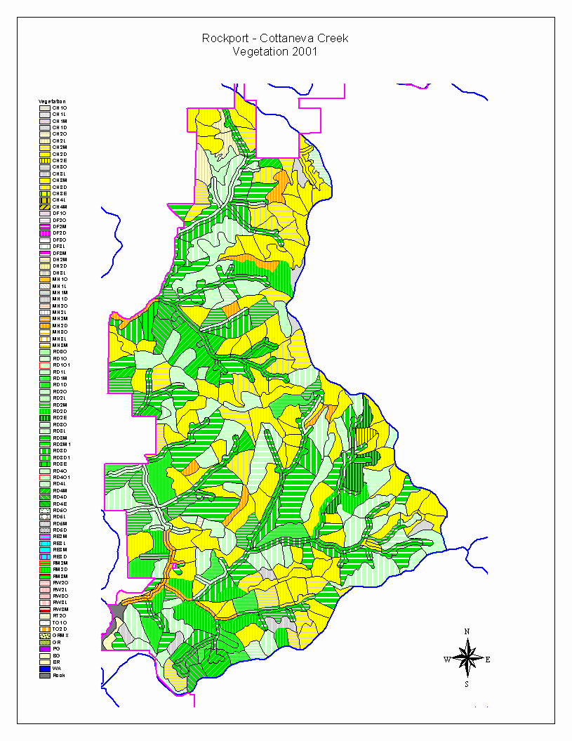
Figure 2. Each stand is assigned a vegetation label interpreted from aerial photos. The vegetation labels are attributed in MS Access and linked to GIS using the stand number.
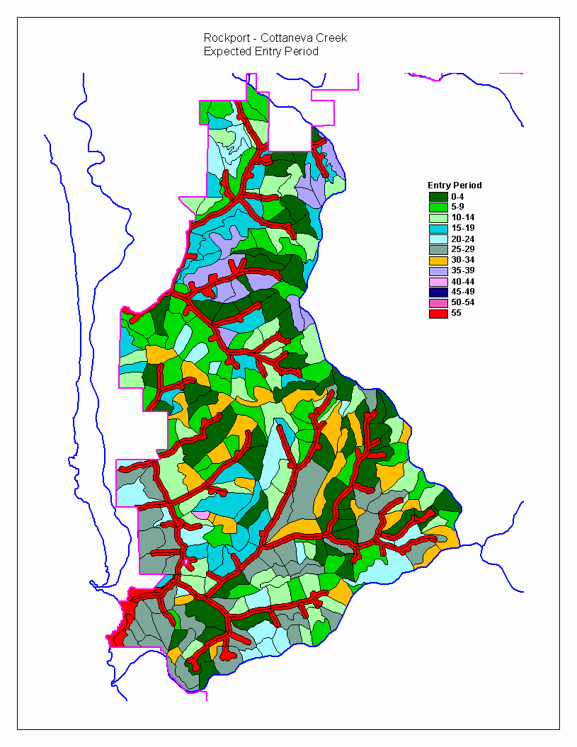
Figure 3. Foresters determine expected entry periods. Consideration is given to the transportation infrastructure, such as roads and bridges, stand condition, and harvest fluctuations in assigning entry periods.
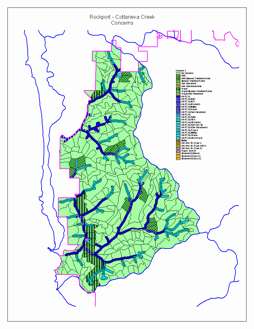
Figure 4. Concern codes originate from data obtained from foresters, biologists, and hydrologists. The concern codes ensure that management activities are appropriate for the concern.
3. Acquire tree lists for each stand through inventory sampling.
The vegetation class assigned to each stand serves as the basis of a stratified inventory. An intensity of 10 to 20 % of a stratum’s acres is sampled for stands that are within 20 years of harvest. A reduced sampling intensity is conducted on open stands, or very young stands that are not likely to be harvested for more than 20 years.
The probability of a stand being sampled is proportional to the size of the stand for a given stratum. A database query generates a table of stands sorted by acres for each stratum. A separate column contains a list of accumulated acres. An interval is selected based on the sum of the acres in the stratum divided by the acres to be sampled in the stratum. A random number between 0 and 100 is added to the interval that selects the first stand to sample in the sorted list, based on the accumulated acres. The subsequent stands selected for sampling are based on adding the interval to the accumulated acres and selecting the stands at the intercept of the accumulated acres and the interval. A minimum of two stands is selected for sampling.
Sampling in the selected stands is conducted using a systematic grid with a random start. Sampling points are located at the intensity of one plot per acre for stands up to 20 acres. For larger stands, an additional plot is located per additional 5 acres. Plots are numbered consecutively and positioned on maps perpendicular to prevailing contours. All skid trails, openings, or other features within the boundaries of the stand are sampled per layout of the plots. Mapped roads are not sampled since an adjustment to gross acres is calculated in the database for all stands.
Sampling is conducted using point samples. All trees with diameters (DBH) six inches or greater are tallied. Species and diameters are recorded for all trees. Height and crown measurements are taken on the first plot and on every subsequent third plot. Heights are measured on all snags, old growth trees, rare species, and trees with broken tops or other unusually poor form. A condition class value is added to separate these trees from other trees in the database. Heights for the unmeasured trees are determined using regression analysis in the database.
A fixed 1/100th-acre plot is also sampled for trees less than six inches. Trees are tallied by species and size class.
4. Determine silviculture strategies.
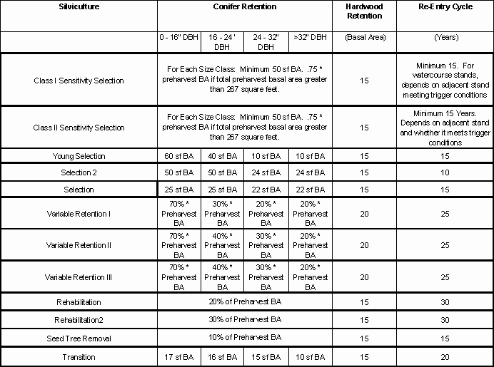
Harvesting strategies are determined prior to modeling activities. The dominant themes in the development of silviculture strategies include harvest intensity, harvest frequency, and biological goals. The strategies include a set of empirical conditions that ensure that the application of silviculture activities is consistent with applicable regulations and with the landowner’s management vision. Harvest initiation includes trigger conditions that consider the stocking levels (basal area) of all species in the stand. Retention levels for all species groups for each silvicultural activity is also defined. In some cases, silviculture strategies are tailored to individual watersheds to address site-specific conditions. Table 2 shows an example of how silviculture strategies are targeted to specific concern codes. It also shows the conditions a stand must meet before initiating a harvest event. Table 3 displays the retention values for conifers and hardwoods and the period until the next entry.
Table 2. Silviculture names, concern codes, and harvest triggers.
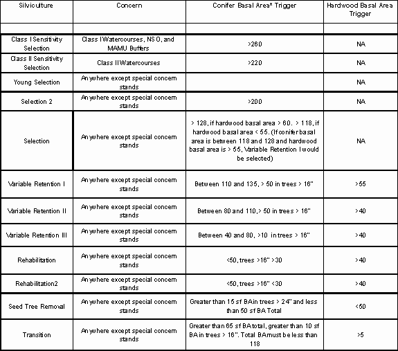
*Basal area is the cross-sectional area of a tree at DBH (diameter at breast height, 4.5’ above the ground). Basal area is expressed here as square feet.
Table 3. Silviculture names, conifer retention, hardwood retention and the re-entry cycle.
5. Perform growth and harvest simulation.
A separate MS Access database is produced for each sub watershed. The database contains the attribute information for the stands in the watershed and the tree list for each stand. The stand number and the area are exported from ArcInfo tables and imported into MS Access tables. The database contains the silviculture triggers and retention levels to be used in the sub watershed.
The tree lists for each stand are grown and harvested in a computer model written in Visual Basic. The growth portion of the model is based on a growth model widely used in the redwood region named CRYPTOS. The growth model consists of several components that include separate functions for:
The tree lists are grown and harvested for each inventory plot in five-year periods. The species, site index, age, live crown ratio, and competition determine the diameter and height increments of each tree.
Stands are harvested when their projected entry period is current with the period being modeled and the stand’s vegetation conditions contain necessary stocking levels to initiate a silvicultural event. Harvest occurs by reducing the individual weight of the tree from the stand’s tree list. The level of stocking required to initiate a harvest event and the intensity of the harvest are based on the silviculture strategies defined in Step 4.
The model outputs periodic tables to the MS Access database. A periodic harvest table is produced that includes the stand numbers, silviculture activities selected, and the estimated volume harvested on a per acre basis for each stand. A periodic tree list table is also produced that includes stand numbers, plots numbers, species, diameters, heights, and weights. The growth and yield model appends small trees to the tree lists to simulate both artificial and natural regeneration. These tree lists can be analyzed to produce a number of reports, including reports showing estimates of projected timber volume and forest structure for each stand.
These tables can be linked to the GIS for a graphical presentation of a time series of timber volume and habitat. Predicted harvest events are presented spatially and display silviculture activities and yields (Figure 5). These graphical displays can be field checked to reveal any errors in the process.
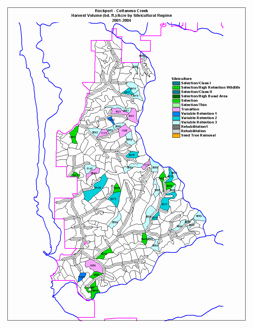
Figure 5. The growth and yield model produces output tables of predicted silviculture activities and yields. These tables are linked to GIS for graphical display.
6. Review model outputs for consistency with management vision.
Foresters, managers, and biologists participate in the review of the model outputs. Graphical presentations from the GIS allow the evaluation of spatial elements related to landscape planning such as habitat connectivity and the use of road networks. Tabular outputs allow review of inventory and harvest trends to determine if the plan achieves the desired environmental and economic goals.
The focus of the biological review is to ensure that habitat levels trend toward, or do not deviate from, desired conditions of the forest, and that special concern areas in the watershed are managed appropriately. This includes mapping habitat conditions over time and reports that indicate changes in the proportions of vegetation structural classes over time. Figure 6 shows the change in forest structural classes over a 50-year planning horizon.
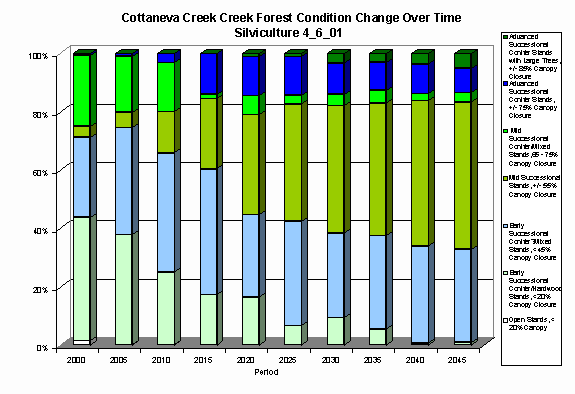
Figure 6. Forest structure changes over a 50-year planning horizon in Cottaneva Creek as the result of planned management activities.
Inventory, growth, and harvest statistics are produced for each watershed. Several of the key indicators that are reviewed include:
Multiple iterations of modeling scenarios can be conducted to smooth harvest trends and test the application of varying silviculture conditions. An example of the inventory, growth, and yield projections is found in Figure 7.
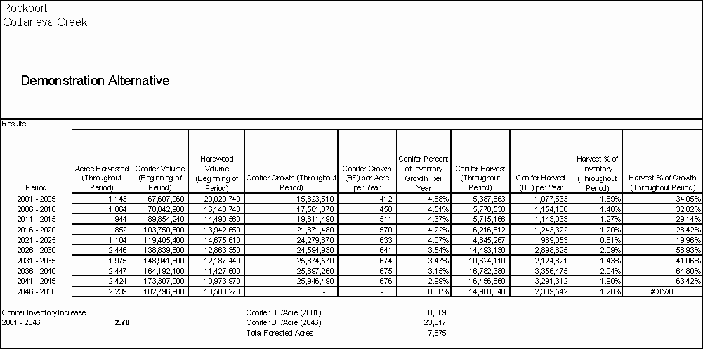
Figure 7. Report showing tabular outputs of growth and yield model. These outputs are reviewed to determine if the scenario is consistent with management goals for the watershed.
7. Integration with other landscape planning processes.
Outputs of the harvest model can be integrated with other aspects of landscape planning. The integration with a road surface erosion potential model is a relevant example.
Road inventory data are collected using Global Positioning Systems (GPS). Data are recorded for road width, surface type (native, rocked, or paved), permanent class (temporary, seasonal, or permanent), prism type, and other attributes. Information is also collected on stream crossings, culverts, landings, and other road-related features. This ground-based survey provides baseline information used during watershed analysis for calculating surface erosion rates from roads. The erosion rates provide estimates of where road associated surface erosion issues are occurring, but changes in timing and frequency of road use may reduce reliability of estimates (MRC 2000). Since stand modeling output provides periodic harvest events and estimated yield, it becomes possible to assess road surface erosion potential in relation to projected harvest activities.
A route-based transportation network and GIS stands coverage are used to develop the road surface erosion potential (SEP) model. Using the stands coverage, label points are converted to a point coverage, and then subjectively "associated" with a route (Figure 8). Stand points are generally associated with the nearest existing road, but topography, stream buffers, and logging methods are also considered.
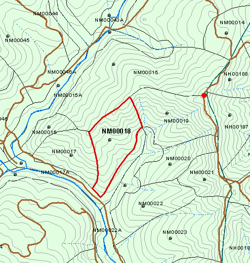
Figure 8. This is an example of subjective stand point association with a route. The stand boundary is outlined in red, and the route-associated stand point is the red dot. Although the road near the bottom of the stand is closer than road to which the stand point was associated, logs would most likely be hauled from the upper road. In this case, a temporary road might be built to access the stand.
After all stand points are moved to a route, a route distance at each point is determined. The route distance to the intersection of each spur road is also determined. These tabular datasets are used to develop a "route path", or the haul route from a stand to a major public road (see Table 4 and Figure 9). Results from these processes are used to calculate the cumulative number of loads that pass over each road segment during each harvest period.
Table 4. List showing an example of a "route path" for truck loads taken from a selected stand. The stand point was associated with route 2081 at milepost 0.30. Route 2081 intersects route 2079 at milepost 1.85, and route 2079 intersects route 2077 at milepost 0.12. This continues until route 2264 terminates at a major public road. Total distance from the stand point to the major road is 14.9 miles.
|
Sequence |
Route ID |
From Distance (miles) |
To Distance (miles) |
|
1 |
2081 |
0.30 |
0.00 |
|
2 |
2079 |
1.85 |
0.00 |
|
3 |
2077 |
0.12 |
0.00 |
|
4 |
2076 |
0.92 |
0.00 |
|
5 |
2096 |
1.10 |
0.00 |
|
6 |
2218 |
9.18 |
0.00 |
|
7 |
2264 |
1.43 |
0.00 |
Total Distance: 14.90 miles
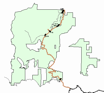
Figure 9. Image showing route path from a selected stand. Brown arc segments are portions of routes used, and gray segments are portions of routes not used. Numbers are distances to intersections corresponding to Table 4.
The SEP calculations are similar to those used in the Noyo River Watershed Analysis (MRC 2000), and are based on guidelines from the "Standard Methodology for Conducting Watershed Analysis" by the Washington Forest Practices Board (WFPB 1995), with modifications for local conditions and to meet the landowner's management objectives.
Most sediment delivered into streams from road surface erosion occurs at watercourse crossings such as bridges, dipped crossings, low water crossings, and watercourse culverts. Cross-drain (or ditch relief) culverts within 200 feet of a stream may contribute sediment from surface erosion and are also included.
Two important parameters used in SEP calculations are the surfacing factor and the traffic factor. The surfacing factor is based on the road tread surface type (Table 5), and the traffic factor is based on the level of road use. Levels of road use are generally grouped into broad categories with associated traffic factors. Traffic factors are assigned to each road segment using criteria in Table 6.
Table 5. Road tread surfacing factors. Values represent tons sediment per year per acre of road tread.
|
Surface Type |
Surfacing Factor |
|
Paved |
1.8 |
|
Rocked |
12 |
|
Native |
60 |
Table 6. Descriptions of road use categories and associated traffic factors. Adapted from Noyo River Watershed Analysis (MRC 2000).
|
Road Use Class |
Road Use Categories |
Road Use Description |
Traffic Factor |
|
I |
Mainline road with heavy traffic |
These roads are actively used and maintained for log haul traffic. |
20 |
|
II |
Mainline roads with moderate traffic |
These roads are used for heavy log haul traffic 2-3 times each decade. |
2 |
|
III |
Seasonal Roads |
These are tributary roads that receive moderate log haul traffic 1-2 years each decade and light traffic the remainder of the time. |
1.2 |
|
IV |
Temporary Roads |
These roads receive moderate log haul traffic 1-2 times per every 1-2 decades with little to no use in between. |
0.61 |
Intensity of road use is a critical factor in road surface erosion modeling. Reid and Dunne (1984) note that "road surface erosion is extremely sensitive to traffic levels." Assigning static values to road segments does not reflect changes in road use associated with long-term timber harvest activities. To account for such variation, the model uses a relationship between number of loads of logs (as a surrogate to road use) and traffic factor.
Previous studies (Reid and Dunne 1984, Bilby et al 1989) indicated log-type relationships between road use and sediment production. Using this assumption, a log-normal curve is fit to the number of loads per segment and traffic factor (Figure 10), with the range of the traffic factor between 2 and 20, corresponding to road use classes II and I, respectively, from Table 6. For this relationship, moderate use is described as 1 load per day and heavy use as 4 loads per day. In coastal Mendocino county, the logging season is approximately 200 days. This would equate to approximately 200 and 800 loads per year for traffic factors 2 and 20, respectively. The traffic factor (TF) is represented by the following equation:
TF = 0.9186 * e0.0039 * loads
where loads is an average number of loads for a road segment per year. Note that the output from the stand harvest model is in 5-year blocks. Load estimates are divided by 5, giving an average number of loads per year. When the calculated traffic factor is greater than 20, a value of 20 was assigned, and when the calculated traffic factor is less than 2, the traffic factor assigned during watershed analysis is used.
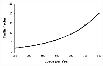
Figure 10. Graph showing log-normal relationship between loads per year and traffic factor. The equation of the line is TF = 0.9186 * e0.0039 * loads, where loads is number of loads per year.
The surface erosion potential is calculated for each contributing road feature described previously and then summed for the entire road.
Various outputs can be used to assess road use changes in relation to stand harvesting. Figure 11 show stands scheduled to be harvested and associated road use for nine 5-year harvest periods from 2006 though 2050. Stands are coded by the estimated number of loads to be harvested from each stand, and roads are coded by the estimated number of loads to pass over each arc segment. The figures clearly show varying road use during different harvest schedule periods.
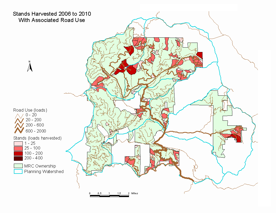
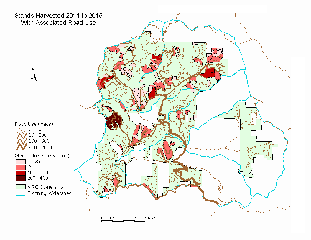
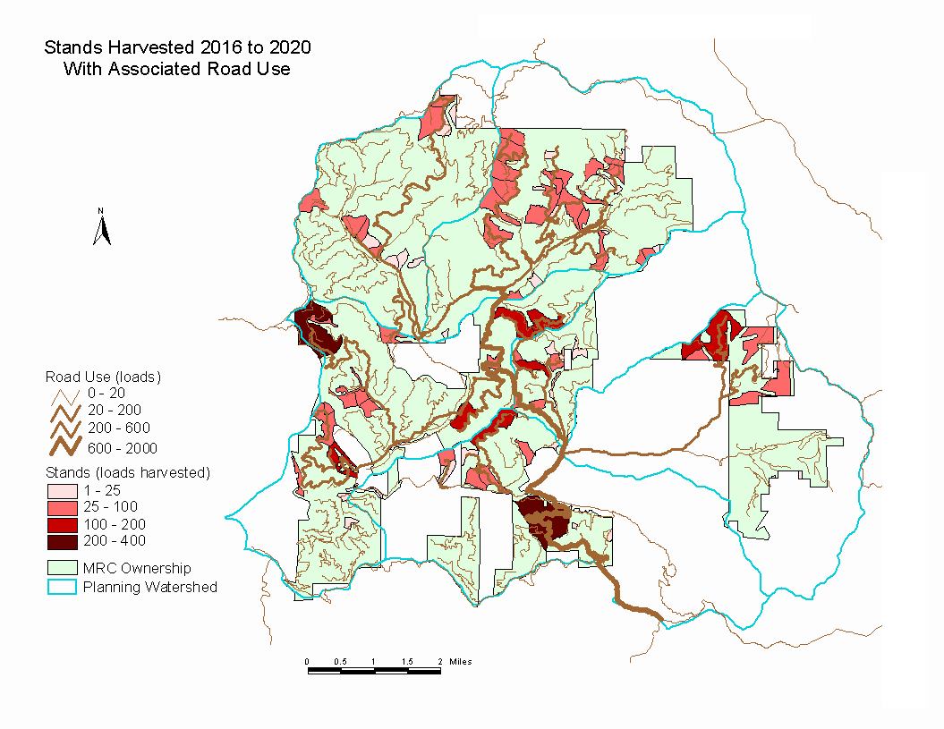
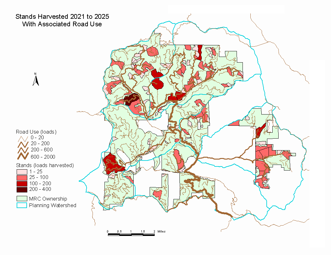
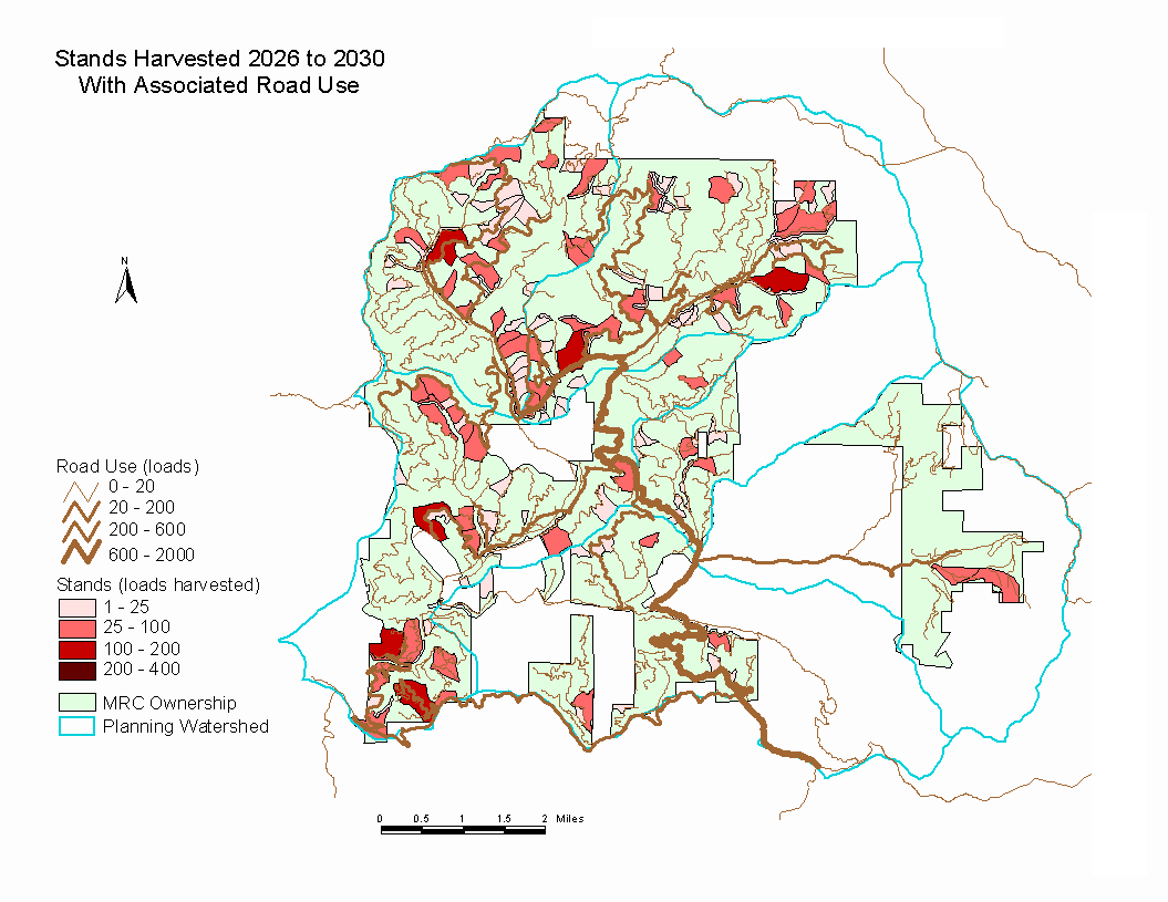
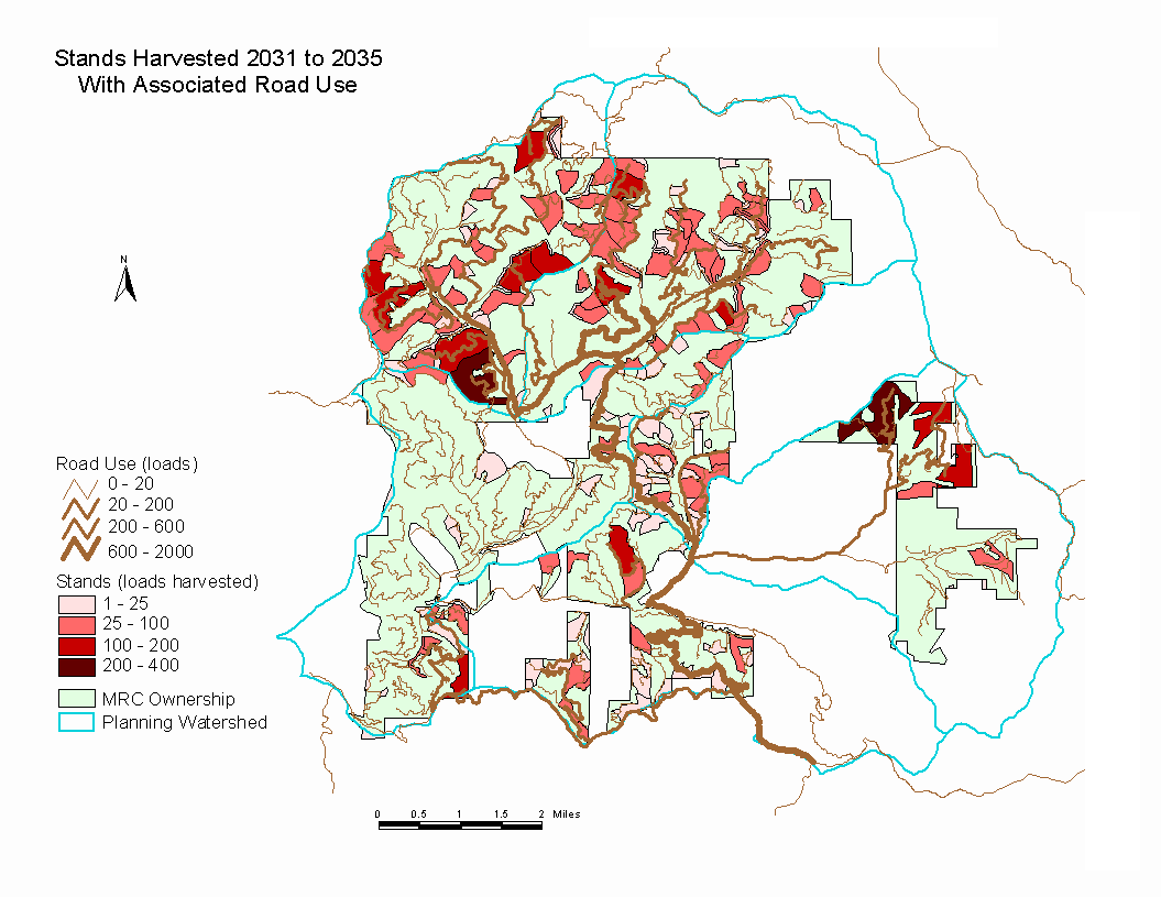
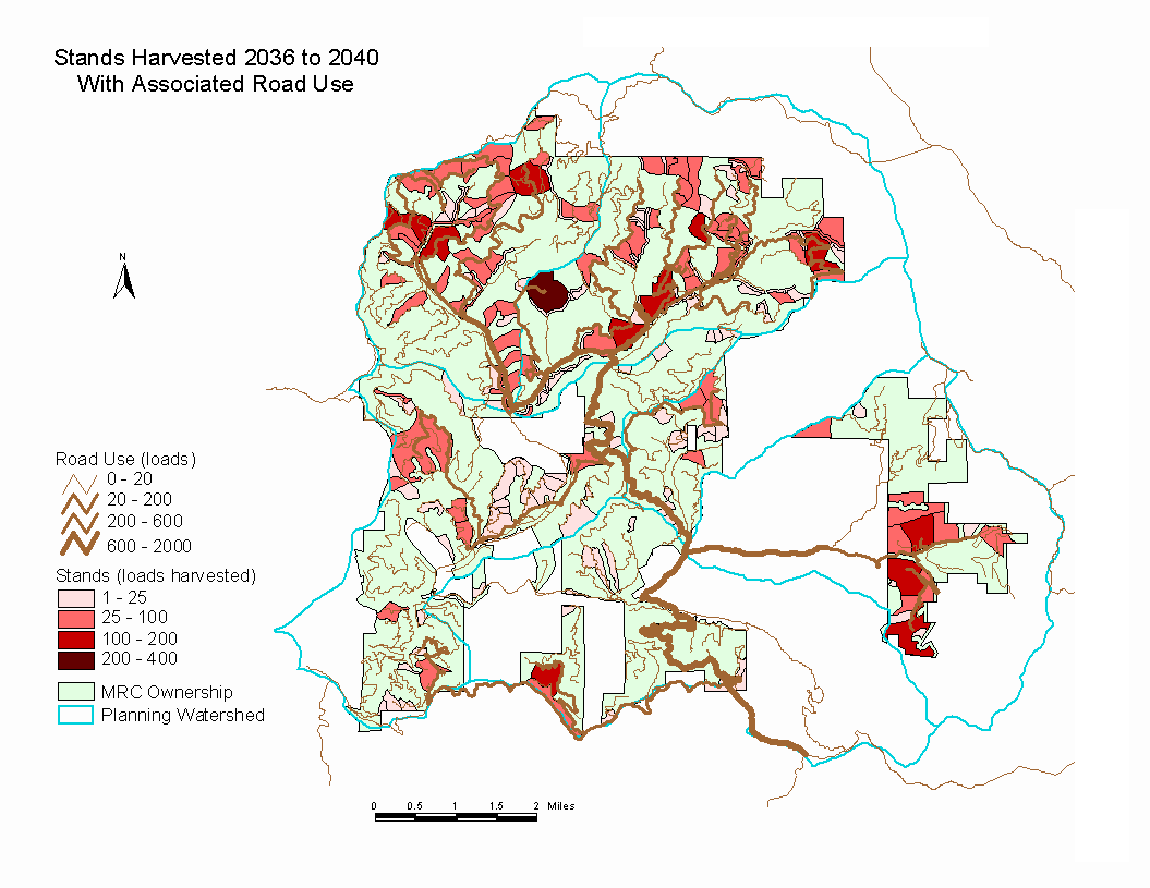
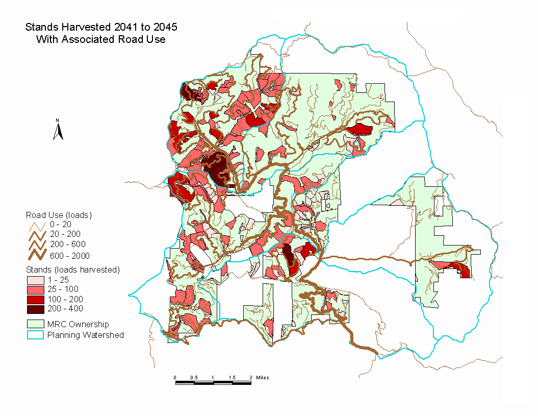
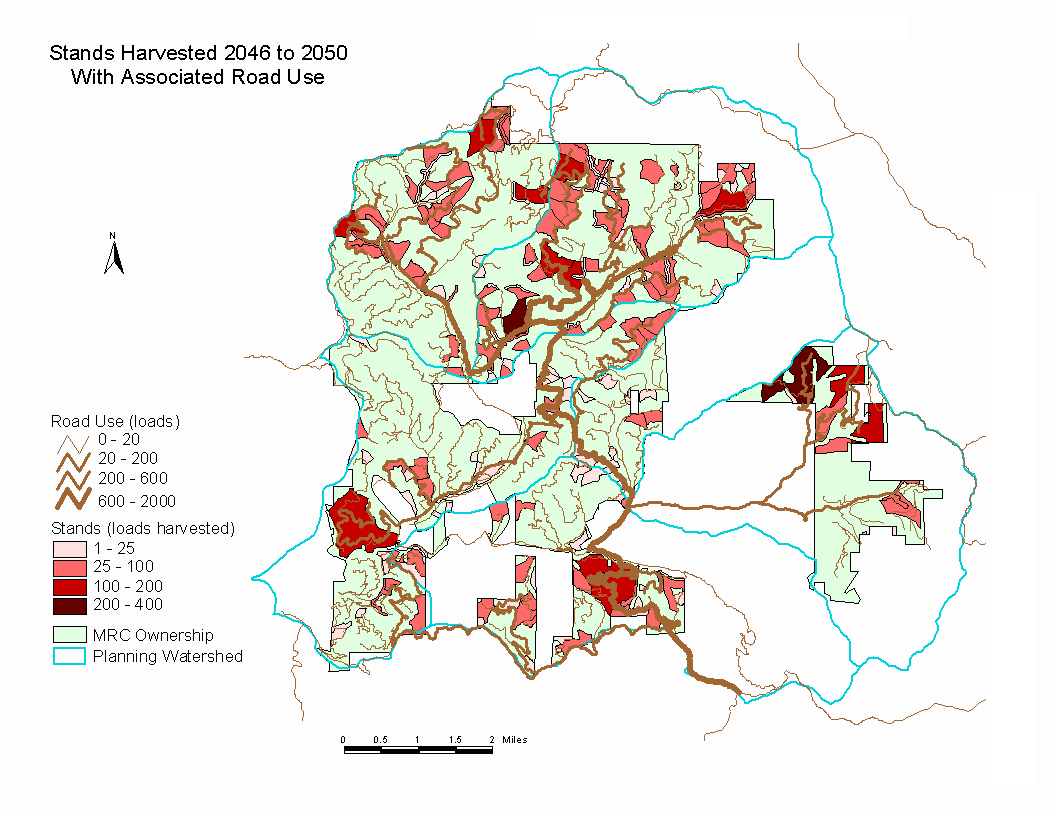
Figure 11. Stands scheduled to be harvested and associated road use for nine 5-year harvest periods from 2006 though 2050. Images demonstrate changes in timing and road use intensity in relation to projected harvest activities.
Figure 12 shows a map of culverts and crossings categorized by the estimated surface erosion potential for each of these features for one 5-year period from 2021 to 2025. This map allows visual assessment of surface erosion potential in relation to other features such as watercourses. This allows users to prioritize sediment management projects.
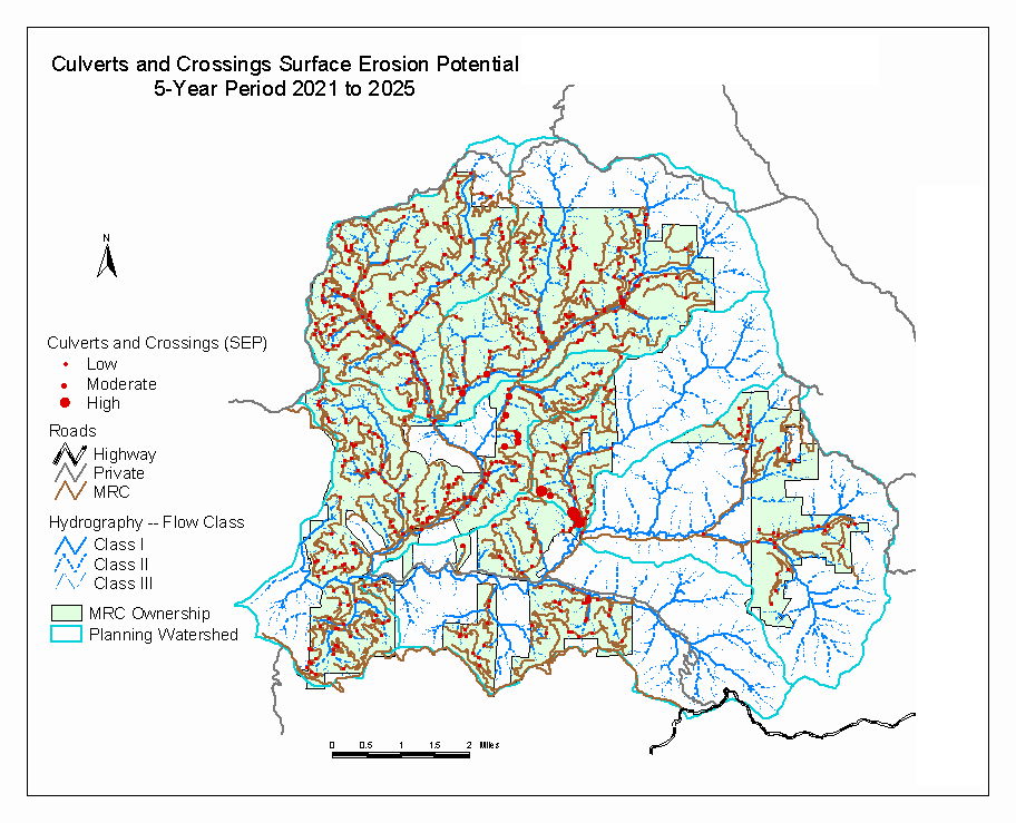
Figure 12.
Map showing culvert and crossing locations. Features are classified by the estimated surface erosion potential (tons sediment per year) for one 5-year harvest period 2021 to 2025.Other applications derived from this model allow alternatives to be examined to reduce sediment-related impacts. For example, an MS Access form was created to allow a user to model "what-if" scenarios involving changes in surface type. The user can change surface type (e.g., from native to rocked) for individual arcs or an entire road, and then recalculate the surface erosion potential for that road. This can be repeated for multiple roads, and then surface erosion potential can be summed for planning watersheds. These types of what-if scenarios are useful for cost-benefit analyses to help evaluate timing and location for sediment management projects.
Stakeholder participation is critical to successful implementation of management plans. Landscape models developed from ground-based data help to build stakeholder confidence. These types of models give managers the ability to assess implications of various management options, and help to weigh ecological and economic considerations. The tools we have presented enable resource managers to assess spatial and temporal impacts at a watershed level and are valuable aids in landscape planning.
We would like to thank Mike Jani and Nancy Budge of Mendocino Redwood Company for providing the space and confidence to allow tools to be developed.
We would like to thank Chris Surfleet of Mendocino Redwood Company for providing the data from watershed analysis used in the sediment model.
We would also like to thank the foresters, cruisers, biologists, and analysts whose participation allow the process to occur.
Bilby, E.B., K. Sullivan, and S.H. Duncan. 1989. The Generation and Fate of Road-Surface Sediment in Forested Watersheds in Southwestern Washington. Forest Science. Vol.35, No.2
Mendocino Redwood Company, LLC (MRC). 2000. Noyo River Watershed Analysis. Calpella, CA
Reid, L.M., T. Dunne. 1984. Sediment Production From Forest Road Surfaces. Water Resources Research. Vol.20, No.11
Washington Forest Practice Board (WFPB). 1995. Standard Methodology for Conducting Watershed Analysis. Version 3.0. WA-DNR Seattle, WA.
Wensel, L.C., B. Krumland, and W.J. Meerschaert. 1987. CRYPTOS user’s guide: The cooperative Redwood Yield Project Output Simulator. Agricultural Experiment Station, University of California, Division of Agriculture and Natural Resources. Bulletin 1924. 89 pp.