Michael Strager, Peter Claggett, Emily Clifton, Jerald Fletcher, Paul Kinder, Don Kemlage, Randy Pomponio, Todd Schroeder, Matt Sherald, Jacquelyn Strager, Charles Yuill
Contents:
Introduction
Structure of Extension
Water Quality Analysis
Landscape Indicators
Wildlife Habitat Indicators
Potential Landscape Change
Model
Discussion
References
Author Information
Abstract
As our landscape continues to change in response to increasing human population and demand for natural resources, we can expect more stressors on water quality, wildlife habitat, and ecosystem processes as a whole. Integrating concepts derived from landscape ecology and the hydrologic sciences with geospatial data and algorithms promotes sustainability through support of local and regional decision-making and planning. By using a customized ArcView application in conjunction with geographically referenced data, decision-makers, planners, and local environmental stewards can assess the current conditions of their watersheds, counties, and/or regions as well as visualize and quantify the potential impacts of future changes to their landscapes.
Achieving sustainability in the future will in part depend on our ability to predict and manage landscape changes and the effects of those changes on natural systems. To better understand landscape change and assist in decision support, the Canaan Valley Institute (CVI) and the Natural Resource Analysis Center (NRAC) at West Virginia University have developed an ArcView GIS extension to evaluate the impacts of landscape changes using indicators related to water quality, wildlife habitat, and overall landscape condition. Users of this extension can interactively incorporate changes to the landscape or model potential landscape changes from new development. This extension allows users to compare indicator values based on current landscape conditions with indicator values based on user-defined or modeled future landscape conditions. Potential applications for this tool include cumulative impact assessments, landscape ecological analyses, comprehensive planning efforts, and overall natural resource management. This document first outlines the conceptual structure of the extension and then describes the modeling components.
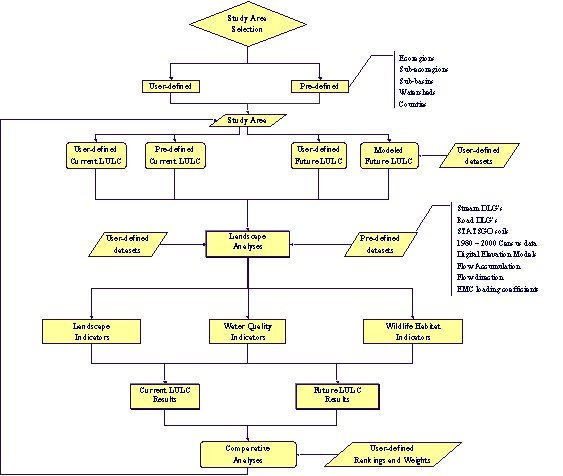
This extension was created using the Avenue programming language, runs within ArcView 3.2, and requires the Spatial Analyst extension. The goal was to create a user-friendly interface with advanced analysis capabilities. Figure 1 below outlines the basic structure of the extension.
Figure 1. Basic Structure of Extension

After loading the Landscape Analyst Extension, the first step for the user is to use the extension’s interface to load the appropriate data layers into a configuration file. Data layers such as land cover, streams, and elevation are specified and can be referenced by an XML file for subsequent use. After the data layers are loaded, the study area selection and analysis functions are available to the user.
The analysis functions are performed on a user-defined study area.
The study area can be defined interactively by drawing a graphic on the
screen around a feature, or it can be selected as a subset of a larger
data layer. For example, the study area selection graphical user
interface allows users to choose from a listing of watersheds, counties,
eco-regions, townships, stream names, or permitted discharges. Conversely,
the user can interactively delineate a study area by on-screen digitizing.
After a study area is selected, the program will zoom to the selected feature
and enable an assortment of general and specific analysis tools for the
user. Analysis tools include:
The water quality modeling component of this extension uses Expected Mean Concentration (EMC) values for land use and cover classes. The EMC values are derived from field data that can be directly linked to the land cover classes. It should be noted that there are factors other than land cover that contribute to nutrient export. However, these factors are rarely known with certainty. Some of the factors that may vary across watersheds and in turn may affect the EMC results include:
Main data inputs include land cover, runoff and cumulative runoff grids. The classes of the land cover grid can be aggregated to match loading rates for individual classes. For example, in using National Land Cover Dataset 30m land cover grid, the 15 classes listed in parentheses below are generalized to fit the loading rate information available for pollutants.
Table 1. Expected mean concentrations (EMCs) for land use/cover
classes (Sample data for Pennsylvania Watersheds, Nizeyimana et. al. 1997)
|
|
|
|
|
| Urban |
1.89
|
0.009
|
166
|
| Open/Brush |
2.19
|
0.13
|
70
|
| Agriculture |
3.41
|
0.24
|
201
|
| Woodland |
0.79
|
0.006
|
39
|
| Barren |
3.90
|
0.10
|
2200
|
| Wetland |
0.79
|
0.006
|
39
|
While the values listed above were calculated for Pennsylvania Watersheds by Nizeyimana et. al. (1997), the Landscape Analyst allows the user to enter specific loading rates corresponding to similar or alternate land cover classes. The ability to test the sensitivity of the rates by changing values also provides insight into boundary thresholds for water quality. In addition to nitrogen, phosphorous, and suspended solids, other pollutants can be modeled using this methodology such as biological oxygen demand, cadmium, chromium, copper, mercury, nickel, and zinc. For a more detailed listing of potential parameters see CH2M HILL (1993), Novotny (1997), and Raird (1996).
Once nutrient export coefficients are entered, they are multiplied by the amount (area) of a given land cover type. They are used in simulation to estimate the probability of increased nutrient loads from land cover composition. Depending on the pollution parameter, two new themes are added to the View’s table of contents. One of the modeled results will be in mg/L and one in Kg/Yr.
The raster data that drives this analysis consists of “hydrologically” conditioned Digital Elevation Models (DEMs), flow direction, and flow accumulation grids. The input data required to develop the hydrology grids include a USGS 30 meter DEM grid, an annual precipitation grid, and stream hydrology. The first step is to create a stream coverage that is fully dendritic, i.e. a layer that represents the drainage network with a fully connected set of single lines (Saunders, 1999). This includes using a single centerline segment instead of left and right bank lines for major rivers and streams. It also includes removing any stray non-networked streams and lakes or ponds. On ponds or lakes fed from drainage, a centerlined stream arc (artificial path) through the water body should be used. For more details on vector hydrology pre-processing refer to Saunders, 1999.
The processing method of reconditioning the DEM for hydrological modeling uses four main steps; (1) rasterize fully dendritic hydrology and thin the raster grid cells, (2) assign sink filled DEM elevation values to the grid cells of the raster stream network, (3) alter the stream network raster cells to ensure that elevations progress in a descending order toward the outlet(s), and (4) use a fixed elevation difference of 20 meters between the stream network raster cells and the surface DEM cell values. The reconditioned DEM after steps one through four was then used with the Esri GRID module functions flowdirection and flowaccumulation.
Using the flow direction grid, watersheds were delineated upstream of each USGS gauging station. The 30-year average annual precipitation was found for the contributing area above the gauge. A linear relationship was created by regressing the 30-year annual average flow rates at the USGS gauges to the 30-year annual precipitation value. This linear relationship was then used to create grids of runoff and a cumulative annual runoff grid. A grid of stream flow can also be generated from the runoff grids. The methods used to create these runoff grids followed the work of Saunders and Maidment (1996).
The water quality modeling results are subject to the following limitations. The transport of pollutants is considered to be conservative (values are averaged over changing flow conditions only) so that no loss or decay of pollutants is considered. This modeling is essentially landscape-based fate transport advection dispersion that uses a runoff grid and flow grid for downstream concentrations and loads. This assumes that streams have the same hydrogeometric properties (stream slope, roughness, width, and depth) and also assumes that the streams have the same ecological rate constants (reareation rates, pollution decay rates and sediment oxygen demand rate). Other limitations are that the modeling does not consider infiltration, or ground water flow additions nor does it include atmospheric conditions such as evapotranspiration.
The landscape indicators included with this extension serve as indirect measures of terrestrial and aquatic habitat integrity and threats to terrestrial and aquatic habitats. For example, forests along streams serve to stabilize stream banks, slow flood waters, filter out nutrients and pollutants from overland flow, and provide shade and shelter to aquatic fauna. Streams lacking forested buffers may suffer from increases in temperature, non-point sources inputs of nutrients and sediments, and altered flow regimes.
The output for each landscape indicator is a single value for any selected study area. Percentage values represent the proportion of the selected study area containing forest cover, edge habitat, etc. The majority of the landscape indicators are calculated based on satellite derived land cover data and digital elevation models with a resolution of 30 meters. For base mapping, line data representing roads and streams is derived from 1:100,000 scale TIGER files or from the National Hydrologic Dataset. Due to the coarse resolution of these data, it is not advisable to calculate these indicators on study areas less than 10,000 acres in extent.
The landscape indicators included with the extension are:
The percent of forest that is contained in the largest patch of forest in a study area is an indirect indicator of forest fragmentation. “If the forest is in one continuous patch, then the area of the largest forest patch equals the total forest area. If the largest patch is smaller than this expected value, then fragmentation has occurred and the remaining forest is discontinuous.” (Jones, et al., 1997). Forests become fragmented when a large continuous forest tract is broken up into smaller forest patches i.e., a forest stand surrounded by non-forest areas. Over time, the clearing of forest for harvesting timber, mining, planting crops, or constructing homes fragments forested areas into smaller, isolated tracts. The fragmentation of large contiguous forest tracts creates remnant forest patches and increased edge habitat. Newly opened forest gaps and increased edge may attract generalist predators, competitors or brood parasites (e.g., Brown-headed Cowbird) that often adversely affect interior forest birds (Laurance and Yensen, 1991). Edge effects also include the increased vulnerability of remnant forest patches to disturbances, such as invasive exotic species, fire, wind, and flooding (Lord and Norton, 1990). Knowledge and concern about forest fragmentation has increased over the past decade due to growing evidence that habitat fragmentation is directly related to the loss of regional and global biological diversity.
The percent forest edge habitat indicator is an indirect estimate of amount of edge habitat available in a selected study area. Forest patches contain edges along the forest/non-forest borders. Forest edges provide ecotones where food sources, habitat, and energy sources are enhanced. The diversity of species inhabiting the forest edge is typically higher than the diversity of species found deep within large forest tracts or within non-forest areas such as grasslands because along the forest edge, some forest and non-forest species coexist and are accompanied by species that are unique to forest edges. However, the diversity of species along forest edges is often higher because exotic invasive species are attracted to those areas. The fragmentation of large forest tracts into smaller ones and the perforation of large forest tracts by human activities result in the creation of more forest edge habitat. While some animals, particularly game species, may benefit from an increase in edge habitat, other animals such as interior forest birds may be adversely impacted. Too much edge in the wrong places provides access for forest pests, disease, unnatural predators, invasive plants and animals, and pollution. In addition, trees along the forest edge are subjected to greater variations in microclimate and greater storm damages.
Forested riparian areas stabilize stream banks, slow flood waters, and filter out some nutrients and pollutants from overland flow before they enter a stream. Streams through forested land uses have been shown to receive few pollutants from the landscape. They also receive the benefits of natural energy, pollution buffering, shading and food sources from the forests. Notwithstanding point sources of pollution, streams that flow through forests are typically high quality streams. In contrast, streams lacking a forested buffer may suffer from increases in temperature, non-point sources inputs of nutrients and sediments, and altered flow regimes. This indicator assumes that all class 1 – 4 roads and all mapped streams are 30m in width and that intersecting road and stream pixels represent either roads crossing streams or roads immediately adjacent to streams. Road pixels adjacent to stream pixels are not counted in the analysis.
The human use index represents the proportion of a selected study area with “human” land uses such as urban, agriculture, mining, transitional, and grassland land uses. High proportions of human land uses are indicative of environmental problems such as enhanced peak stormwater flows containing high levels of nutrients, sediment, and other contaminants, soil erosion, and aquatic and terrestrial habitat loss.
Roads serve as animal movement corridors and both connect and fragment the landscape. Roads may disrupt, restrict, or enhance the dispersal of plants and animals. They are a source or conduit of noise, dust, and pollutant runoff. Roads improve human access to the land and facilitate development. The impact of roads on the landscape is a function of road size, traffic volume, and type of use. Roads constructed near watercourses pose potential risks to water quality and may alter stream hydrology. Run-off from roads contains vehicle-related chemicals and pollutants such as sediments and nutrients, oils and greases, salts, etc. that may enter adjacent watercourses. Run-off from roads also may increase peak stream flows.
Population density and change serve as indicators of the degree of current human interaction with and modification of the landscape. Landscapes with dense human populations are likely to have been highly modified by humans and are typically classified as urban, residential, and agricultural land uses. Landscapes experiencing high population growth rates are likely to be undergoing land use change, e.g., from forest to agricultural/residential and from agricultural to urban/commercial. Population densities also tend to correlate with recreational use pressures and water consumption and waste production levels. This indicator assumes that population densities are proportional to road densities and that no humans live beyond one kilometer from paved roads.
Soil loss potential is an indirect measure of potential soil erosion from agricultural lands based on the Universal Soil Loss Equation (USLE) as developed by the U.S. Department of Agriculture. The USLE is based on soil texture, slope, land cover, precipitation, and cropping practices. Soil erosion reduces the productivity and increases the turbidity and sediment load in streams. Severe erosion problems can lead to the complete loss of productive topsoil and the loss of benthic stream organisms, which form the backbone of biotic support for fish. Soil is essentially a non-renewable resource. It takes over 500 years to naturally produce an inch of topsoil in humid, temperate climates such as predominate in the northeastern United States
The assumptions in calculating these parameters include:
The wildlife indicators incorporated into the Landscape Analyst extension include species-specific models including a Louisiana Waterthrush habitat model, more general models such as the Bird Community Index, and species presence, absence, and richness based on USGS BRD Gap Analysis Program data.
The Louisiana Waterthrush habitat model is based upon the assumptions that this bird species prefers forested riparian areas composed of deciduous, mixed, or woody wetland vegetation along first through third order streams. These forested riparian areas must be > = 300m in length, and have elevation < 1000m. Optimally, Louisiana Waterthrush prefer habitat that meets the above requirements and is also surrounded by 315 hectares (90% of 350 ha) of forest composed of deciduous, evergreen, mixed, and woody wetlands.
The Bird Community Index (BCI) provides a comprehensive measure of terrestrial habitat quantity and quality. O’Connell, et al. (2000) developed the BCI as an indicator of habitat disturbance applicable to the Mid-Atlantic Highlands region. The development of the BCI is based on regional studies of guilds of songbirds, e.g., groups of birds requiring similar habitat, prey, and other conditions for survival. Bird species are considered a good indicator for ecological condition, since each species differs in its sensitivity to habitat conditions (e.g. food, shelter), and since birds are readily found and easily identified. Many bird species’ traits can be linked to specific environmental conditions, making the BCI a useful environmental indicator.
The BCI is a numerical rating or score that indicates overall ecological condition across the landscape. The BCI is calculated based on land use patterns within 200 acre windows. Poor ecological condition is associated with less than 28% forest cover while good or excellent condition is associated with greater than 87% + forest cover. Edge effects for disturbed areas larger than 5 acres are also included.
The USGS BRD Gap Analysis Program is an ongoing effort to predict and analyze wildlife habitat and species distributions on a state level. Currently, all Mid Atlantic states (MD, PA, WV, VA) in the CVI service area have complete or nearly complete wildlife distribution datasets. The Landscape Analyst extension will make use of available Gap datasets in several ways. The extension can produce lists of species predicted to occur in user-specified areas. Associated Gap datasets can also be used to predict species lost or gained in an area following potential land cover changes modeled using the extension module described in the next section.
Potential Growth and Landscape Change Model
This module of the Landscape Analyst extension also allows users to model potential landscape changes through on-screen digitizing and subsequent land use reclassification within ArcView or through an interactive development model.
The interactive development model relies on the cost path algorithm within ArcView’s Spatial Analyst extension. A cost surface is created for the study area based on landscape variables such as existing or proposed transportation networks, slope, hydrology, and land cover. Users then have the ability to weigh each of the model parameters to test its sensitivity to user preferences or to test the significance of each parameter. The potential growth model simulates urbanization emanating along a least cost surface from user-defined growth centroids. Using general topographic constraints, the model extends likely development away from the user specified locations. This is primarily driven by infrastructure of existing roads, elevation constraints with slope, and likelihood of conversion assigned to different land cover classes. The development model does not consider any zoning, socioeconomic or community influenced factors that may be involved in development patterns and growth.
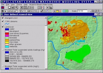
With new boundaries established for likely growth, the effects on the water quality, landscape, and wildlife indicators can be rerun to examine the affects. For example, the southern barren area as shown in Figure 2 (below) is obviously contributing much to the total suspended solid loading (345 mg/L and 1,369,888 Kg/Year) at the highest points. If the southern strip mine were converted to grassland by re-vegetating the landscape, what would be the decrease in total suspended solids? To evaluate this question, we would simply change the land cover grid by digitizing in the polygon of change and attributing it with the changed land use and merging it into the land cover grid as shown in Figure 3.
Figure 2.
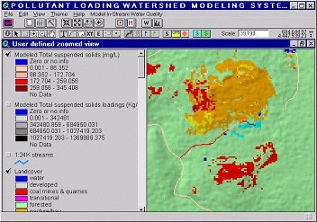
Figure 3.
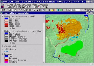
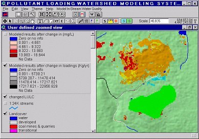
After rerunning the model with the changed land cover location (coal mine and quarry (barren) changed to revegetated grassland), we observe that total suspended solid concentrations decreased to 18 mg/L and 22,956 Kg/Year at the highest points in the watershed. The updated results are shown in Figure 4 A and B (Strager et al. 2000).
Figures 4a - 4b
 |
 |
This extension differs from other landscape and water quality screening models (such Fragstats, Attila, PLOAD) in the ability to spatially simulate landscape change. Not only can land cover classes be changed (i.e. from deciduous forest to clearcut) but the extent, location, and size can be altered as well. This customized editing ability allows for more directed modeling of future conditions. In addition to the manual editing of land cover change, the potential development modeling component automatically generates maps of potential expansion of existing development based on topographic features and logical constraints.
As with any modeling effort, the water quality, wildlife, landscape, and land cover change modeling incorporated in this extension have several assumptions that must be taken into account. Despite these limitations, by placing these modeling capabilities in an ArcView extension, we have gained the important advantage of easily analyzed visual output. The open architecture of the extension easily allows more detailed datasets as part of the configuration files. Users can easily incorporate improved land cover datasets with the extension as they become available.
The Landscape Analyst extension developed by this cooperative effort takes a broad scale view to assessing regional environmental quality in terms of water quality, land use, and landscape change. The extension uses indicators to calculate and summarize statistically relevant data. The indicators for water quality, landscape pattern, and wildlife habitat were not designed to be evaluated in absolute terms, rather, they provide useful relative comparisons of conditions for differing study areas and land use scenarios. The extension combines many useful tools and models together in a comprehensive package designed to be useful in regional ecological modeling, monitoring, and assessment efforts.
CH2MHILL, 1993. Urban Stormwater Pollutant Event Mean Concentrations and Annual Runoff Coefficients for Calculation of Annual Pollutant Loads – Task F1 – “Pollutant Loadings”, DERM Stormwater Management Master Plan, Phase 1 (C-9 East Basin Study), Prepared for the Metropolitan Dade County Department of Environmental Resources Management, Miami, FL.
Jones, K.B., K.H. Riitters, J.D. Wickham, R.D. Tankersley, Jr., R.V. O’Neill, D.J.Chaloud, E.R. Smith, and A.C. Neale. 1997. An ecological assessment of the United States Mid-Atlantic region: A landscape atlas. EPA/600/R-97/130. U.S. Environmental Protection Agency: Washington, D.C.
Laurence, W. F. and E. Yensen. 1991. Predicting the impacts of edge effects in fragmented habitats. Biological Conservation 55: 77-92
Lord, J. M., and D. A. Norton. 1990. Scale and the spatial concept of fragmentation. Conservation Biology 4(2):197-202
Nizeyimana, E., B. M. Evans, M. C. Anderson, G. W. Peterson, D. R. DeWalle, W. E. Sharpe, J. M. Hamlett, B. R. Swistock, 1997. Quantification of NPS Pollution Loads Within Pennsylvania Watersheds. Final Report Prepared for Pennsylvania Department of Environmental Protection, Bureau of Water Quality Protection. Environmental Resources Research Institute, University Park, PA.
Novotny, V., and H. Olem, 1994. Water Quality: Prevention, Identification, and Management of Diffuse Pollution, van Nostrand Reinhold, New York.
O’Connell, T.J., L.E. Jackson, R. P. Brooks, 2000. Bird Guilds as Indicators of Ecological Condition in the Central Appalachians. Ecological Applications 10(6):1706-1721.
Raird, C., M. Jennings, D. Ockerman, and T. Dybale. 1996. Characterization of Nonpoint Sources and Loadings to Corpus Cristi Bay National Estuary Program Study Area, Corpus Cristi Bay National Estuary Program/USGS/NRCS, CCBNEP-05, Table IV.9.http://arpon.tamucc.edu/Library/FinalReports/pdf/CCB05.pdf.
Saunders, W. K. and D. R. Maidment 1996, A GIS Assessment of Nonpoint Pollution in the San Antonio-Nueces Coastal Basin, Center for Research in Water Resources Online Report 96-1, University of Texas, Austin, TX.
Saunders, W. K. 1999 Preparation of DEMS for use in Environmental Modeling Analysis, In: Conference Proceedings: 1999 Esri User Conference, Environmental Systems Research Institute, Redlands, CA.
Strager, M. P., J. J. Fletcher, C. B. Yuill, J. M. Strager, 2000. Not in My Watershed! – An Interactive Tool to Evaluate Land Use Changes on Stream Water Quality In: Conference Proceedings: 2000 Esri User Conference, Environmental Systems Research Institute, Redlands, CA.
U.S. Environmental Protection Agency. MAIA Project Summary: Birds Indicate Ecological Condition of the Mid-Atlantic Highlands, EPA/620/R-00/003, June 2000.