Abstract: EDAW, Inc. uses GIS technology to analyze a variety of environmental data including archaeology, biology, geology, hydrology, and social impacts. This paper shows how EDAW tackled the problem of trying to analyze biological impacts along a portion of a river that experiences dynamically changing landscape conditions. The setting: a coastal river mouth in an urban area; the project: three alternative alignments for bridge construction; and the problem: calculating biological impacts from bridge construction based on the current conditions would not reflect landscape fluctuations that are evident from historic photographs and that are expected in future years. Our project team was challenged with evaluating the "modern" historic fluctuations that the wetland vegetation communities within our dynamic project setting undergo. The solution: using GIS and Spatial Analyst, EDAW was able to model the "dominant landscape" representing the likely array of vegetation cover within the riparian corridor based on vegetation community patterns evident on historical aerial photographs. This allowed the calculation of impacts associated with each alternative bridge alignment in a manner that reflects periodically changing conditions at the site.
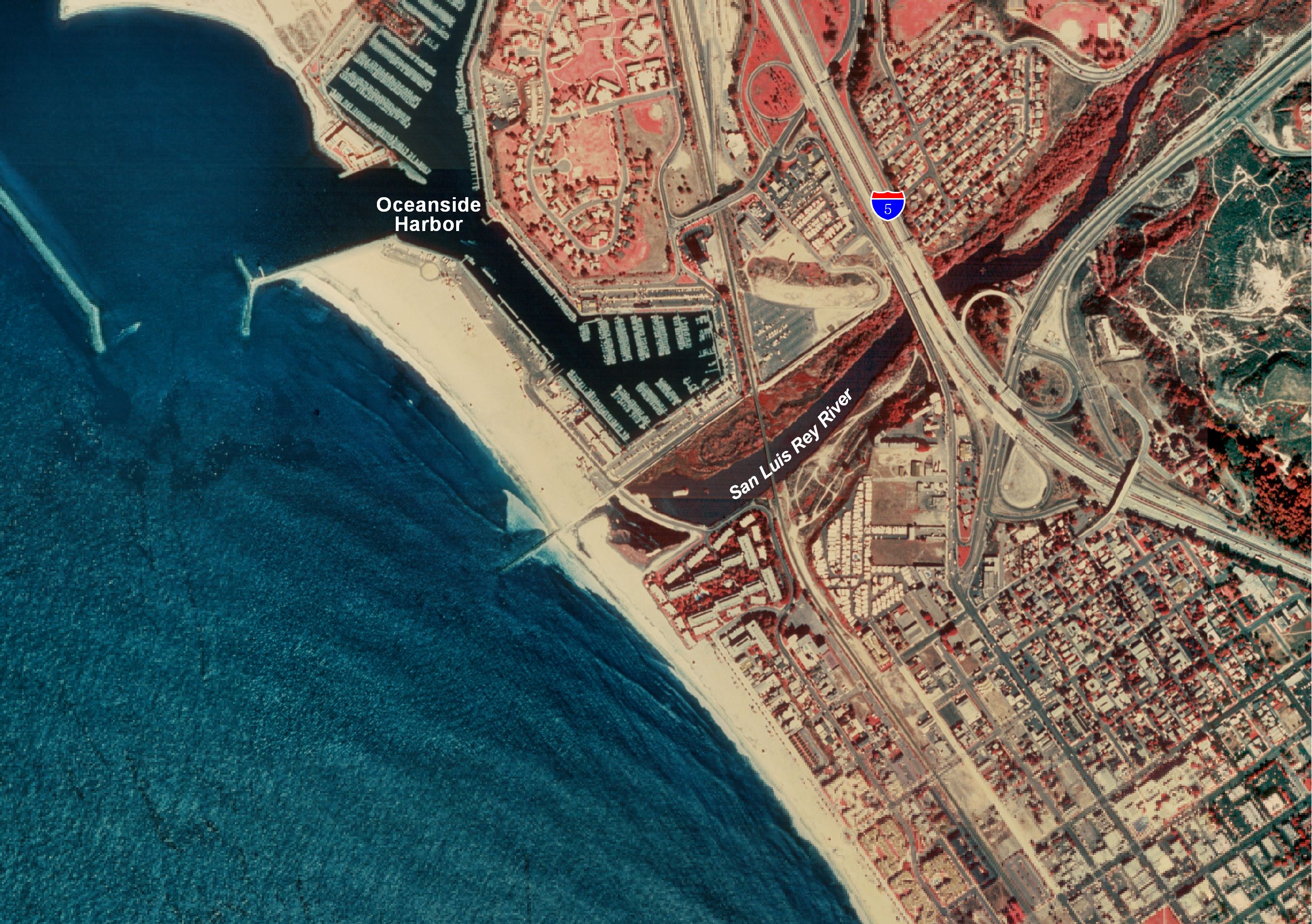
The standard approach to evaluating the impacts to biological resources on a project site is to prepare a thorough mapping of the vegetation communities and other cover types along with other baseline inventories. For most analyses, it is an understanding of the present conditions at a site that is desired. However, some natural communities undergo such significant periodic changes that evaluating a single point in time may not accurately reflect conditions that were present in recent years, and that are expected to return in the near future. Prime examples of fluctuating landscapes are the coastal river mouths in southern California. In general, coastal river mouths are influenced by tidal action and river flows onto the coast. The brackish vegetation communities that develop at coastal river mouths expand with increasing sediment deposition and accretion of biomass, and shrink from the erosional effects of storm surges or the desiccating effects of periodic droughts. Furthermore, the amplitude of the tides and the morphology of the area influence all coastal river mouths. In particular, the site morphology determines the pattern of the river flow, erosion, and deposition. Our project is located at the mouth of the San Luis Rey River in the City of Oceanside (Figure 1). The San Luis Rey River is a major tributary in northern San Diego County that spans 51 miles between its coastal mouth and its headwaters near Mount Palomar. Activities within the watershed that influence this river include an existing dam, sand mining, dairy operations, cattle grazing, intensive agricultural uses, domestic water extraction, and increasing residential and industrial development.
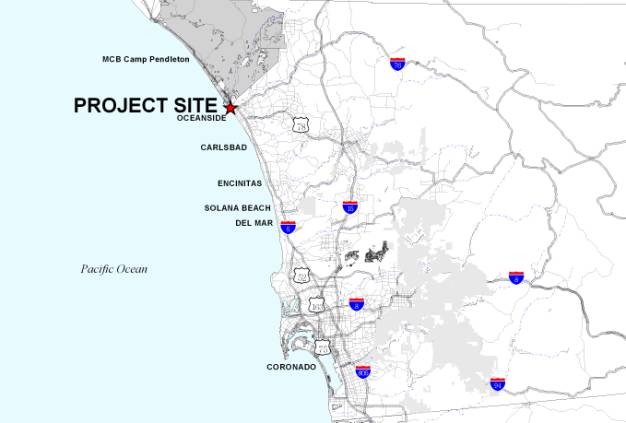
Figure 1
The western-most road crossing of the San Luis Rey River is Pacific Street, an at-grade two-lane road that lies approximately 800 feet adjacent to the shoreline. This river crossing is one of two main access points to the City of Oceanside Harbor and Beach Marina (Figure 2). Culverts under the existing Pacific Street crossing are designed to carry tidal and low flow drainage. However, in order to prevent upstream flooding, the road is designed to wash out during periods of significant rain, and has washed out and been reconstructed six times between 1979 and 1998. Although this crossing is continually subject to washout, the Pacific Street crossing provides a critical access to the harbor and marina area. As a condition of the most recent permit that allowed reconstruction of the current at-grade road, the Regional Water Quality Control Board required the design and development of a permanent bridge.
Figure 2
The project proposes three alternative bridge alignments, which are currently being evaluated under the California Environmental Quality Act. It is our decision to attempt to model the fluctuating conditions at the mouth of the San Luis Rey River, and our solution to problems encountered in this modeling effort, that is the focus of this paper.
Our initial approach for the environmental analysis was to conduct the traditional thorough updated field assessment and inventory of the biological resources within the study area, which includes the area between the beach and Interstate-5. At initial meetings, however, the project team appreciated that the same physical influences that have washed out the road six times in the last 20 years, have also altered the occurrence and extent of the vegetation communities throughout the project study area. The crux of an environmental analysis is an accurate quantification of impacts and a determination of what mitigating measures are necessary. Through initial discussions with the resource agencies, it was decided that the range of conditions that have been present at the site in the last 10 to 20 years should be evaluated in order to understand the dynamics of this river mouth, fairly assess the impacts, and determine what types of mitigation would be feasible to implement within the dynamic conditions of the study area. :
The San Luis Rey River and its watershed have undergone much change since the early 1920's when Henshaw Dam was built near the head of the river. Before development, much of the watershed was used for agriculture, and then in 1964, much of the estuary was dredged to create the Oceanside Harbor (California Coastal Conservancy 1989). The westernmost section of the river, which includes the project area, has been channelized since the 1970's. Aerial photographs pre-channelization and pre-harbor dredging are available and they depict early conditions along the river. However, the project team decided to concentrate our efforts on the recent history of the river mouth when the effects of development have been most constant around the project area. The changes that are evident on recent aerial photographs depict changes directly related to natural tidal influences and storm or runoff flows within a river system that has otherwise been consistently affected by the surrounding land uses.
Color aerial photographs from the last twenty years were viewed, and seven photographs were selected as summarized below:
Aerial photograph date |
Notes |
|
February 22, 1982 |
Pacific Street washed out winter of 1982 |
|
February 11, 1985 |
Pacific Street washed out winter of 1985 |
|
February 5, 1987 |
Pacific Street is present |
|
March 5, 1993 |
Pacific Street washed out winter of 1993 |
|
February 19, 1995 |
Pacific Street washed out winter of 1995 |
|
February 1997 |
Pacific Street is present |
|
March 7, 1998 |
Pacific Street washed out winter of 1998 |
Six of the seven photographs, purchased from Aerial Fotobank, Inc., were scaled to 1"=500'. The 1997 image was printed from an electronic file at 1"=500' to match the scaled color aerials. From the photographs it was not possible to distinguish all vegetation types; however, extrapolating from existing conditions at the site it was apparent where upland vs. wetland vegetation communities were present, and within wetlands, where low- vs. tall-statured vegetative growth occurred. Therefore, vegetation communities and land cover types were separated into four categories: upland, marsh, riparian woodland/scrub, and open water/sand. The boundaries of these broad cover types were then delineated on the seven aerial photographs. Because sensitive wetland habitats are a principal concern of the resource agencies, the historical modeling effort focused on the pattern of wetlands and open water within the riparian corridor.
On acetate overlays, biologists delineated each of the vegetation categories on each of the seven historical photographs (Figure 3). Using an ArchE (36" x 48") Altek Datatab IV digitizer, each of
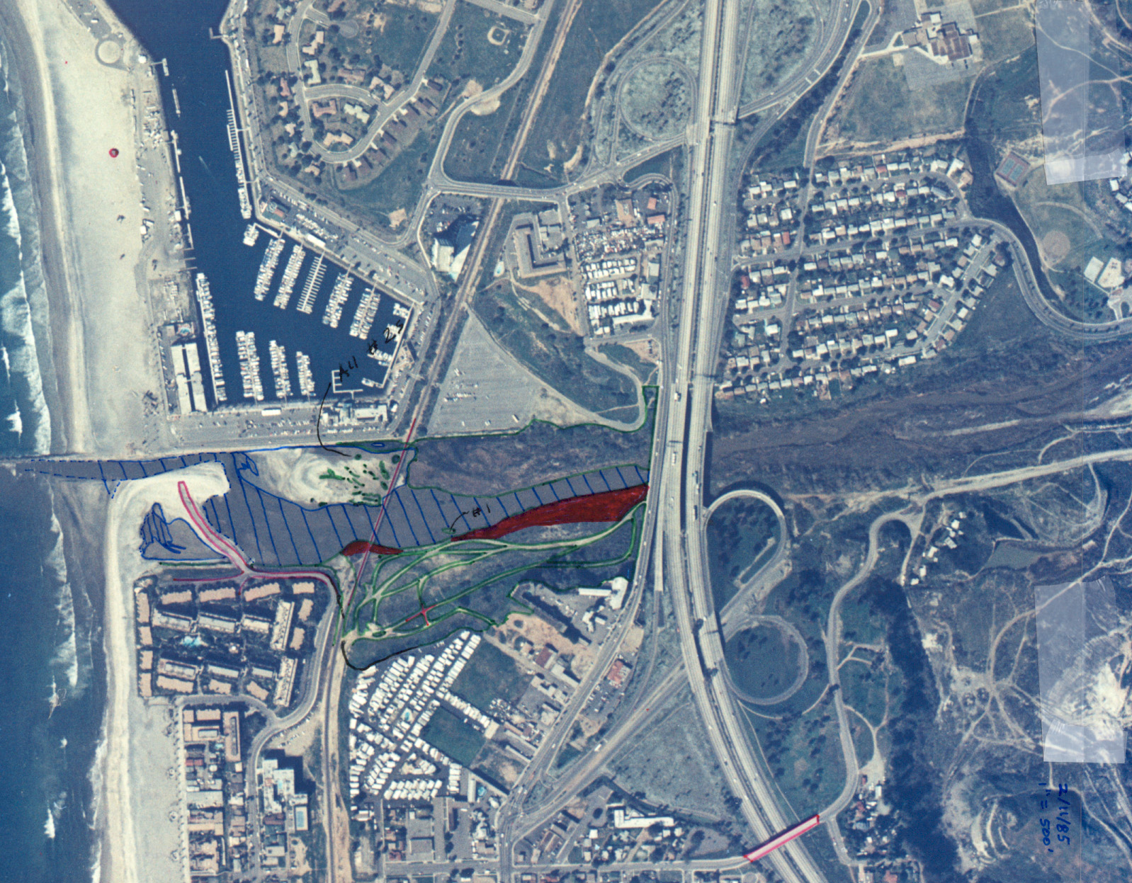
Figure 3
these areas was digitized into ArcView as a shapefile (Figure 4). Registration of the aerial photographs was based on the electronic aerial image of the project area. Project area features that did not vary over time (i.e., freeway interchanges, house roof tops) were used to register each of the aerial photographs. Once areas of vegetation were digitized into GIS, they were verified and updated by project biologists. Final vegetation layers were then completed for each of the seven aerial photographs. Using the final delineated boundaries of upland, marsh, riparian woodland/scrub, and open water/sand from all seven aerial photographs, the team was ready to attempt to model the dominant pattern among these layers.
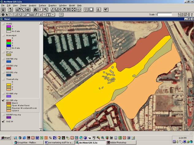
Figure 4
As with any thorough environmental analysis, project alternatives must be analyzed. In our case, the potential effects of three alternative bridge alignments needed to be evaluated in light of our dynamically changing landscape. Each project alternative was provided to EDAW as AutoCAD files that included over 50 layers of data per alternative. To help with the assessment of biological impacts, however, these complex CAD files were imported into GIS using the CAD Reader extension and converted to simpler GIS files. The primary interest for the assessment of impacts was the extent of the project footprint along the riverbank, the placement of bridge piles within the riparian corridor, and the alternative shape of each alignment where it spans the river. Each alternative was coded into these three main feature types and digitized back into ArcView (Figures 5, 6 and 7). Tracking each of these components separately enabled us to identify which component of each alternative footprint would affect which type of riparian habitat as derived by the modeled landscape.
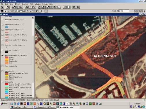
Figure5
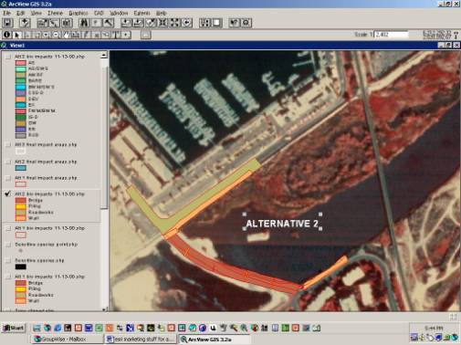
Figure6
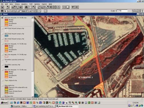
Figure7
Using the Model Builder extension of Spatial Analyst II, we identified the dominant pattern among our seven vegetation layers. First, each layer was converted to a grid using Spatial Analyst. Then each of the three riparian vegetation categories was assigned a numeric code, e.g., Open Water (OW) = "1", Riparian (R) = "2", and Wetland (W) = "3." Once the vegetation layer was converted to a grid, each cell of the grid was represented by one of the three categories (Figure 8).
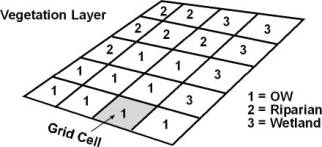
Figure8
Once the historic photographs were converted to the grid pattern and vegetation coding was assigned to each cell in each of the grids, each grid was input into Model Builder and two modeling functions of Model Builder were applied. Using the additive overlay model, the vegetation codes within a specific cell common among the layers were added together, rather than determining which vegetation code was in the majority for that cell. For example, if six of the seven cells for a specific area was coded as "1", and in the seventh layer that cell was coded as "2", then the additive overlay model adds those values together and characterizes the cell as "8", which is the sum of the codes, rather than "1", which would indicate that the code "1" was in the majority (Figure 9).
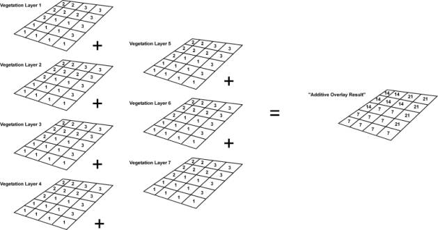
Figure9
Using the weighted overlay model, a similar problem was encountered. With a weighted analysis, the cell values are multiplied by the proportionate influence that is assigned to the layer (Figure 10). In our case all seven layers were weighted equally, so each had an influence of 14.28 percent. Using two layers as an example, if a cell in a particular layer had been categorized as "2" and the corresponding cell in another layer was categorized as "3", the model would multiply the cell by its respective weighting and add those individual values to obtain a weighted and summed output cell value. For this example, the model would calculate 14.28 percent of "2" (i.e., 0.28) and 14.28 percent of "3" (i.e., 0.42), and sum those values together (i.e., 0.70). Moreover, output cell values are rounded to the nearest whole value, which in our example would be 1. This extension, which adds weighted values and rounds the output data, was not the appropriate approach for our modeling need.
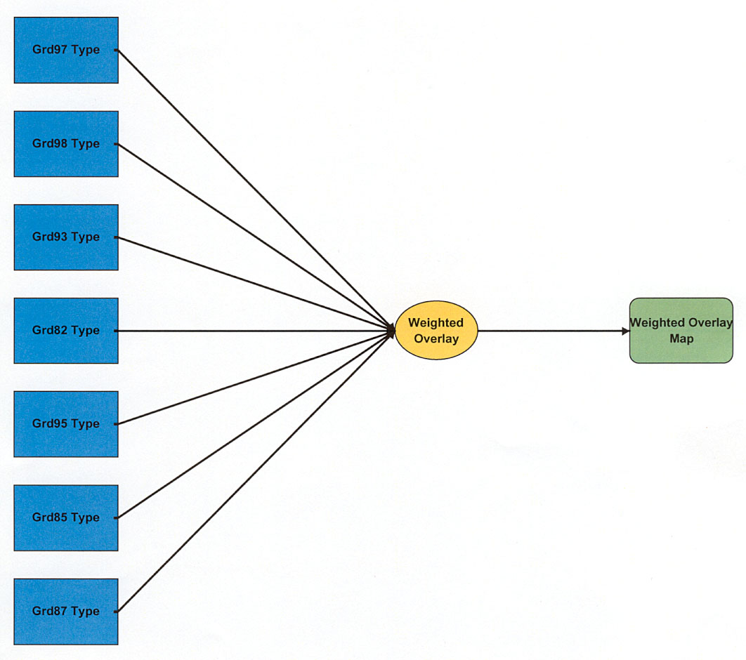
Figure10
Consultation with Esri generated a possible solution. A calculation formula called "majority grid" (Figure 11) was run to determine which numbers (1, 2, or 3) were found to be in the majority for a specific cell among our seven grids.
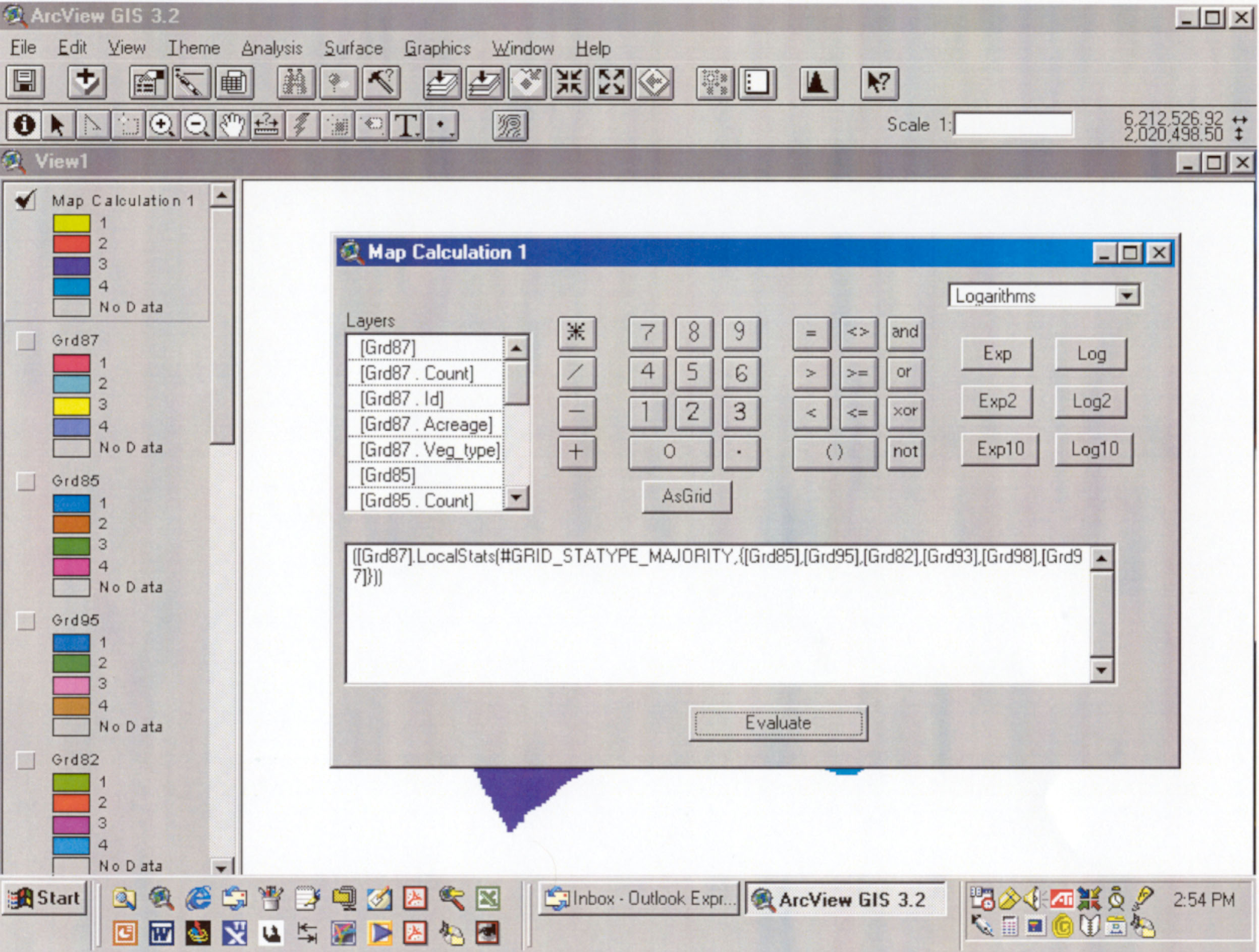
Figure11
This solution worked well except where values tied for a given cell among the grids (i.e., 1, 1, 1, 2, 2, 2, 3, or 3, 3, 3, 1, 1, 1, 2). For tied values, the calculation formula would assign the grid cell "no data." This exercise also demonstrated that although the majority calculation determined the dominant entry for cells where the aerial coverage was consistent among the layers, the calculation will input data from the largest grid available even where that coverage is rare among the layers. The calculation "majority grid" chooses entries from the largest grid even if the majority of grids had no value (i.e., no cover) for that portion of grid cells (Figure 12).

Figure11
Our solution involved a combination of the modeling discussed above. To begin with, the common area of cover among all layers was determined, and each original vegetation layer was "clipped" to this common area. Each year was thus uniformly set to a new constant grid size. The majority grid expression was then re-run for the area that was constant among the layers. Within this clipped area, to remedy the problem with cells that were assigned "no data" because two vegetation codes were tied for being in the majority, a "null grid" expression was run. To run the null grid expression: (1) select the majority grid outcome layer; (2) set the null grid as the "analysis mask" extent; (3) replace "majority" with "sum" in the majority grid theme expression; and (4) re-run this expression on the clipped portion of the original majority grid. This process gave us a grid of those cells with tied values and a sum of the vegetation codes within those tied cells. The two grids were merged using a script called "merged grid" to make one grid that showed all cell values, including the new summed values. Once merged, the cells with summed values were assessed in light of the surrounding cells and recoded with the appropriate vegetation category. This merged and corrected grid was then converted into a shapefile that now represented the dominant vegetation pattern that has been present at the Pacific Street river mouth over the past 18 years. This model of the dominant vegetation pattern was used to calculate impacts for each component of the project (i.e., riverbank, bridge pile, and bridge alignment) among the three alternatives.
Our project is still undergoing environmental review. However, our use of ArcView's Spatial Analyst Extension to model the changing conditions at our project site has been helpful in our discussions with the resource agencies, and in our evaluation of issues related to our environmental analysis including whether mitigation for impacts to biological resources should be located within this river mouth, and if so, what type.
California Coastal Conservancy. 1989. The Coastal Wetlands of San Diego County. 64 pp.
The authors would like to express special thanks to Peter Biniaz and Jerry Hittleman at the City of Oceanside for their assistance in obtaining historical information about the project site, and their support of the GIS modeling; to Talli Carey, the GIS Coordinator at the City of Oceanside for supplying the electronic infrared aerial image for our project area; and to Lisa Pitts, the Technical Support Specialist at Esri for her enduring patience and commitment to helping us solve our modeling challenges.
Paula M. Jacks, M.S., Biologist
Senior Associate
EDAW, Inc.
1420 Kettner Boulevard, Suite 620
San Diego, California 92101
(619) 233-1454
(619) 233-0952 fax
Angela Johnson
GIS Manager
EDAW, Inc.
1420 Kettner Boulevard, Suite 620
San Diego, California 92101
(619) 233-1454
(619) 233-0952 fax