Baltimore's Urban Environment Using GIS and Neural Networks

Abstract

Historical census data for Baltimore MD from 1970-1990 is used to train a neural network model. This same data will be used in a GIS for analysis. A customized graphic user interface (GUI) is developed to allow a user to create user specific data for analysis using GIS. An artificial neural network will use the extracted data to make numerical projections. The project involves database creation and validation, scripting of an artificial intelligence model, calibration of the model from historical data, development of the GUI, making projections, and displaying the results using GIS.

INTRODUCTION

The National Transportation Center at Morgan State University has established a research effort at the School of Engineering to conduct research on Urban Modeling and Design. The premier project of the Center is to integrate GIS data with the analytical techniques of Artificial Neural Networks (ANN).

The methods and techniques developed during the course of this project were based upon the Baltimore City urban area. The city is composed of approximately 203 census tracts organized into 66 neighborhoods. The U.S. census data can be broadly classified into population and housing data. There are numerous sub-fields in these two classes in each data set. The 1970, 1980 and 1990 census data sets were used in this study.

This study looks at the phenomenon of temporal fluctuations of diverse demographic, social and economic characteristics of the test region. It is difficult, if not impossible, to identify change and predict its outcome. Through this study, we will try to identify varying demographic, social and economic characteristics of a targeted urban neighborhood and its adjacent neighbors.

OBJECTIVES OF RESEARCH

The objective is to identify patterns of change exhibited by data for the targeted neighborhood and predict the impact on the adjacent neighborhoods. This data will be analyzed within a Neural Network (NN) program in hopes of identifying trends or patterns. The resultant NN output(s) are to be re-introduced into GIS for spatial analysis. The general thought is to concentrate on a small data set within a defined geographic region.

DATA CREATION

To determine trends and patterns from one period to another required the collection and creation of data. For this study it was decided to create tabular data sets from the 1970 and 1980 U.S. Census tract books (Figures 1,2 and 3). A process that required scanning each census tract book and converting the scanned data into a database format. This was a tedious process that took approximately two to three months to complete.

Figure 1.1970 Census Tract Table

Figure 2.1980 Census Tract Table

Figure 3.1990 Census Tract Table

JOINING DATABASE FILES

ArcView^TM allows the user to load a dBase file into a map by joining it to the attribute table of an appropriate theme. Since this study will look at historical patterns over time, we can join the 1970 and 1980 tabular data to the 1990 attribute table to create an attribute table comprised of thirty years of historic data. When we join our tables to the theme's attribute table, all fields from our table are appended to the attribute table. We need to use these fields of data to symbolize, label, query, and analyze the theme's features. A JOIN operation is based on the values of a field that can be found in both tables. The actual field name does not need to be the same in both tables, but the data types (numbers, strings, etc.) have to be the same. For this study we will join the 1970.dbf and 1980.dbf to our 1990 Census tract theme to create an attribute table comprised of thirty years of historic data. The three tables contain a field that stores the numerical census tract identifier, so we will base the join on this common field.

Steps for Joining Tables

1. In the 1970.dbf table click on the field named "Tract", Figure 1.
2. In the view's Table of Contents, click the "Study Area Theme", and open its attribute table by clicking the Open Theme Table button. In the theme attribute table, click on the field named "Tract", Figure 2.
3. Click the Join button. All fields from 1970.dbf are appended into the attribute table of the Study Area Theme. The fields appear at the right hand side of the table.
4. Repeat steps 1 through 3 for the 1980.dbf table.
5. We now can use these fields to symbolize the Study Area Themes.

For this study, we have collected the following data:

• Hampden Boundary map
• Remington Boundary map
• Baltimore: Past, Present and Future - Trends and Projections - Feb 1997
• The Baltimore Neighborhood Fact Book
• Census Tract Comparability Tables from Census Tracts and Block Numbering
• 1970 Census Tracts, Baltimore, Md
• 1980 Census Tracts, Baltimore, Md
• 1980, 1970 Community Profiles Baltimore City data by Census Tracks
• 1980, 1990 Regional Planning Districts and Census Tracts
• 1990 Census Tracts maps
• 1990 Baltimore Neighborhoods Statistics map
• 1990 Community Profiles Baltimore City: Demographic, housing, health, educational, income, public assistance and crime data by Census Tracts
• 1990 Census Data by Neighborhood Book #13, Census News
• 1990 Census Data by Neighborhood Book #12, Census News 1990
• 1991 Neighborhood Service Centers/Police Districts map

GRAPHICAL USER INTERFACE DEVELOPMENT

A GUI has been developed to streamline the processes needed to truncate a large data set so that the data may be exported out of ArcView^TM for numerical analysis and then imported back into ArcView^TM and joined to the original data set for comparison. To illustrate, we show the first GUI (Figure 4) of the Urban Model Builder leads the user into a step-by-step (Figure 5) procedure for opening a theme.

Figure 4.Opening the Urban Neighborhood Model Dialog

Figure 5.Opening the Urban Neighborhood Model Dialog

To make this task possible, it was first necessary to build a database for use in ArcView^TM containing all of the Census information from these different years. As information from successive years was added to the database, it became unmanageably large. To make a computer application that will be sufficiently user-friendly it is necessary to substantially truncate the data set.

Figure 6.Selecting geographic area(s) of interest

However, it is desirable to allow all of the data to exist so that the user has some degree of flexibility as to which geographic region they wish to perform analysis on and what data they choose to use for their analysis. This is shown in Figures 6 and 7.

Figure 7.Selecting field(s) of interest

The GUI now exports the selected data to a text file for importing back into ArcView^TM as shown in Figure 8.

Figure 8.Saving selected data as a text file

After saving the text file, the user is asked to name the theme as shown in Figure 9, and save it as a new shape file.

Figure 9.Saving a New Shapefile

In Figure 10 the final output of the selected criteria to analyze using ArcView^TM is shown.

Figure 10. Final Theme Created from shapefile

Artificial Neural Network

The temporal trends for the urban area are often observed through key indicators. The conclusions drawn from such indicators as to whether the region is in a state of rise or decline, are often subjective. This arises out of the inter-relationship and dependencies between the observable and measurable characteristics of the region. These relationships, being complex in nature and non-deterministic or 'fuzzy' to a certain extent, are best captured through a pattern recognition approach, as in Artificial Neural Networks. The existence of 'hard' data from census tracts from 1970 - 1990 is well suited as a training data for such a network. We perceive the surrounding environment based upon certain patterns. We need to understand these patterns and learn their meanings. If the patterns are stable we tend to believe that over time it is possible to predict what that patterns future might become. ANN will allow us to process a large amount of data where as it would be impossible otherwise.

Basics of Discrete Modeling

Consider a test area, which is an urban area with well-defined boundaries, as shown in Figure 11. Let us assume that this test area is divided into a finite number of divisions. In the model presented here, the total urban area represents an isolated neighborhood and the sub regions (A-F) are Census Tracts comprising the neighborhood. U.S. Census data is available by census tracts. For each census tract, demographic and housing data are available. Examples of Census data sheets from the 1970, 1980 and 1990 censuses are shown in Figure 1 - 3.

Figure 11. Schematic of a Typical Urban Area

For this study we will use 1970, 1980 and 1990 US census data for race and housing to train the NN. We will predict the 2000 distribution of race and housing and display the results using GIS.

We have generated the GIS results in Figures 12 through 21.

Results

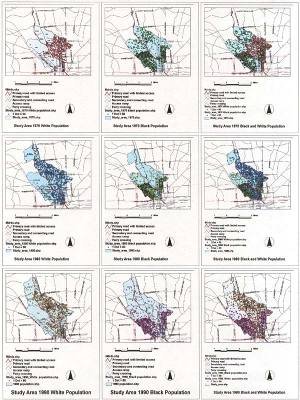
Figure 12 indicates white population distribution along highway I-83. These results are extracted from 1990 US census and displayed using ArcView^TM.

Figure 12. White population distribution along highway I-83

Figure 13 indicates black population distribution along highway I-83. These results are extracted from 1990 US census and displayed using ArcView^TM.

Figure 13. Black population distribution along highway I-83

Figure 14 indicates black and white population distribution along highway I-83. These results are extracted from 1990 US census and displayed using ArcView^TM.

Figure 14. Black and White population distribution along highway I-83

Figure 15 indicates white population distribution along highway I-83. These results are extracted from 1980 US census and displayed using ArcView^TM.

Figure 15. White population distribution along highway I-83

Figure 16 indicates black population distribution along highway I-83. These results are extracted from 1980 US census and displayed using ArcView^TM.

Figure 16. Black population distribution along highway I-83

Figure 17 indicates black and white population distribution along highway I-83. These results are extracted from 1980 US census and displayed using ArcView^TM.

Figure 17. Black and White population distribution along highway I-83

Figure 18 indicates white population distribution along highway I-83. These results are extracted from 1970 US census and displayed using ArcView^TM.

Figure 18. White population distribution along highway I-83

Figure 19 indicates black population distribution along highway I-83. These results are extracted from 1970 US census and displayed using ArcView^TM.

Figure 19. Black population distribution along highway I-83

Figure 20 indicates black and white population distribution along highway I-83. These results are extracted from 1970 US census and displayed using ArcView^TM.

Figure 20. Black and White population distribution along highway I-83

Figure 21 is a side-by-side comparison of black and white population distribution along highway I-83 from 1970, 1980 and 1990.

Figure 21. Side-by-side comparison of black and white population distribution along highway I-83 from 1970, 1980 and 1990

Future Research

The development of an urban neighborhood model of Baltimore City to assist decision - making, by applying GIS and artificial intelligence would continue this research effort. Using historic data from demographic, social and economic factors, research in understanding the influence of the various factors within individual neighborhoods should assist one in determining the impact of these factors on adjacent neighborhoods. It will therefore become a decision - making analytical tool in the prediction of demographic, social and economic changes from the analysis of historic data. This approach requires extensive data collection techniques, data extraction and data integration methods with GIS, decision - making applications, and artificial intelligence.

Acknowledgements

The research reported in this paper was supported by a Faculty Research Grant from the National Center for Transportation Management, Research and Development. NTC is part of the USDOT University Transportation Centers Program. The Center was established by Congress under the Intermodal Surface Transportation Efficiency Act of 1991 (ISTEA), and reauthorized in 1998 by the Transportation Equity Act for the 21st Century (TEA-21). The NTC is located on the Morgan State University campus in Baltimore, Maryland.

The research reported in this paper was supported by Greenhorne and O'Mara, Inc. Facilities, Housing, and Community Living Division, and its Geographic Information Services Division, both located in Greenbelt, Maryland.

References

Author Information

• Tony E. Graham
  Doctoral Student, Department of Civil Engineering
  Morgan State University, Baltimore, MD
  443.885.1442
  410.319.3843
  tgraham@eng.morgan.edu
  
• Indranil Goswami, Ph.D.,P.E.
  Assistant Professor, Department of Civil Engineering
  Morgan State University, Baltimore, MD