As terrestrial landscapes become increasingly fragmented by human activities, a predictive approach for estimating animal abundance that accounts for spatial heterogeneity is needed to guide habitat management and conservation. Our spatial modeling approach, developed as an ArcView GIS extension, incorporates empirical data on animal responses to habitat edges and predicts abundances under various land management scenarios. Inputs to the model include habitat maps and animal density response functions. The latter describe animal density along a habitat gradient between adjacent habitat types, allowing us to generate predicted animal abundance maps.
The detrimental effects of habitat fragmentation on animal populations are widely documented (Whitcomb et al. 1981, Robinson et al. 1995), however, the development of practical tools to predict the effects of fragmentation and design appropriate mitigation efforts has progressed slowly (Saunders et al. 1991, Wiens 1995). Current models typically apply average animal density values to thematic maps of vegetation or habitat. However, it is known that many animals avoid or exploit boundaries or "edges" between habitats. That is, the habitat adjacent to a focal habitat patch can influence its quality, which is sometimes referred to as the matrix effect (Forman and Godron 1988). Our spatial modeling approach incorporates empirical data on animal edge responses into a model that predicts animal abundance, reproductive success or other response variable within a landscape context (Sisk and Margules 1993, Sisk et al. 1997, Sisk et al. 2000).
The Effective Area Model (EAM) is designed to provide a predictive tool to link field and remotely sensed data in a landscape model that permits comparison of the impacts of alternative land use strategies on animal populations. It is constructed so that managers can create their own hypothetical scenarios and explore the potential outcomes of alternative management strategies.
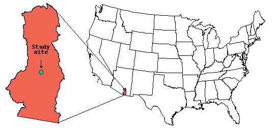
The model has been tested on birds and butterflies in northern Arizona pine forest and southern Arizona riparian habitats. In this paper we use butterfly data, collected within the Upper San Pedro River watershed in southern Arizona (Figure 1), in the EAM to predict the number and distribution of individual butterflies in one section of the San Pedro River. We then compare EAM predictions with the predictions of a null model that ignores edge and matrix effects. The results show that incorporating edge effects can yield important differences in the estimated animal population size in two of the three habitat types modeled. Another way this model improves on most earlier models is its consideration of error. We are testing techniques for estimating the impact of both spatial error, such as from remotely sensed data, and error from field estimates.

Riparian areas are a major reservoir of both plant and animal diversity in arid ecosystems (Naiman et al. 1993). The San Pedro is the last, major, free-flowing river in Arizona and supports a diverse plant and animal community compared to the surrounding desert. The San Pedro originates in Sonora, Mexico and flows north into southeast Arizona. The San Pedro River is located within a transition zone between Sonoran and Chihuahuan deserts and supports vegetation communities found in both ecotypes. The Nature Conservancy has declared the San Pedro riparian corridor one of the twelve "last great places of the western hemisphere" in terms of ecological diversity and much of its course lies in a national riparian conservation area. American Rivers, a non-profit group, has listed the San Pedro fourth on its 1999 list of the top ten endangered American rivers. The main threats to the San Pedro River are groundwater pumping and urban sprawl (Stromberg et al. 1996), so its conservation is a sensitive issue that has received national attention (1999 May 4, NY Times). Recently, a binational initiative to preserve the San Pedro was announced by the U.S. Secretary of the Interior.
The San Pedro River has undergone dramatic transformation since European settlement in the mid-1800s. At that time, the river was marshy, not-incised, and supported only scattered trees with some forested reaches (Stromberg 1998). Grazing and cultivation had become common by the early 1900s and a combination of events at the turn of the century, including tree-removal and drought followed by a series of floods caused major channelization (Stromberg et al. 1996). This created a two-tiered flood plain with primary and secondary zones dominated by different vegetation communities. Since the turn of the century, the vegetation structure has changed dramatically from a primarily open marsh/grassland to a highly heterogeneous landscape increasingly dominated by edges between trees, shrubs, and remaining open habitat.
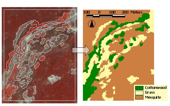
The primary flood plain is now characterized by gallery forests dominated by Fremont cottonwood (Populus fremontii) and Gooding willow (Salix goodingii). In general, the width of the primary riparian area ranges from 50 - 300 m. These gallery forests have a great deal of variation in their degree of canopy closure, varying from almost completely closed to primarily open habitat with a few, scattered trees. This primary flood plain supports several wetland obligate species including Juncus sp. and Scirpus acutus (Stromberg et al. 1996). The secondary flood plain generally exists on a raised terrace and occurs between the primary flood plain and the surrounding desert scrub. The height of this terrace ranges from 1 - 8 m above the primary flood plain. The width of the secondary riparian zone varies from 0 - 1000 m. This zone of vegetation also exhibits a tremendous amount of variation. The area ranges from completely open habitat to areas with mixed grass and mesquite (Prosopis velutina) to areas dominated by ōbosquesö (forests) where the mesquite forms a closed canopy and tree height can reach 10 m. These bosques often have large openings in the canopy where a more developed herbaceous layer is likely to persist. Our study focuses on a section of the San Pedro River, within the San Pedro Riparian National Conservation Area, where there are patches of cottonwood within the primary flood plain surrounded by open habitat, and the secondary riparian area is dominated by bosques with several open areas embedded in the mesquite (Figure 4). It is the edges between the forested (both cottonwood and mesquite) and open habitat that form the basis of our modeling efforts for this paper.
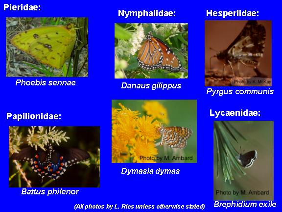
Because of its location and the lush habitat surrounded by desert, the San Pedro River exhibits high diversity and abundances of many taxa, including butterflies. In fact, it has one of the most diverse butterfly fauna in North America. Over 100 species of butterflies have been found on the upper San Pedro. In our surveys to date, we have identified over 70 species, a few of which are shown in Figure 2.
In this raster-based spatial model, an animal density grid is created by applying animal density response functions to the closest edge (habitat boundary) from each cell. In addition, the model includes an optional statistical method to map variance in animal density estimates. Model inputs include a habitat map and animal density response functions. The model was developed in ArcView GIS version 3.2 (Esri, Redlands, California) using the Spatial Analyst extension and Avenue scripting language. It will likely be recoded for use in ArcGIS 8.1. The current version of the model and a user manual containing step-by-step instructions is available from the EAM web site.
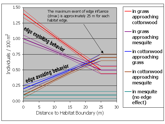
Density response functions can be derived from field data, the published literature, or created based on a known range of responses in order to explore whether edge responses are likely to be an important factor in a particular landscape of interest. For this example, edge response functions represent a composite based on preliminary data from several butterfly species found on the San Pedro River. Our preliminary results indicate that butterflies exhibit positive, negative, and neutral edge responses, and that responses often are evident within 20 ¢ 30 m from the edge.1 Our hypothetical species, therefore, shows a positive edge response at two edge types, a negative response at two edge types, and no edge response at two edge types (Figure 3). All edge responses occur within 25 m of the edge. It should be noted, however, that we are currently collecting detailed field data on 15 to 20 butterfly species on the San Pedro, and this data will be used to derive rigorous, continuous edge functions.
Using the EAM requires edge response functions for each species of interest at each edge type. Obviously, collecting these data requires a large field effort which may not always be feasible. When field data are unavailable, information from the published literature can be used. Many species of birds have had sufficient data collected that their edge response functions at several edge types are known. For species where less information is available, life history characteristics could be used to make inferences about which edge responses are most likely.
One of our goals in this project is to rigorously test the idea that certain life history characteristics correlate with general edge response functions. If there are certain life history characteristics that predict edge responses, then these general responses (or a reasonable range of responses) may be used in lieu of actual field data. The advantage of this approach is that scenario testing may proceed before costly field collection. If the simulations indicate that edge responses are likely to be an important factor in the dynamics of the region, then expending the resources to collect field data may be indicated.
In order to obtain the most informative results, field data should be collected from the focal landscape for each species of interest. Field studies designed to collect data for edge responses can take different intensity depending on the desired accuracy of output (Sisk et al. 2000). Data should be collected at all edge types present in the system that will be included in the modeling effort. At the very least, data should be collected at two edge distances, ōedgeö and ōinteriorö. However, because the distance that edge responses extend into a particular habitat type are often not known, we advise having several distance classes.
For San Pedro butterflies, we have erected 100 m transects comprised of 10 x 10 m contiguous quadrats. However, most field studies will not be able to collect data at such a fine scale and this scale of data collection may not even be necessary. Perhaps if we had used only two edge distance classes ("edge" and "interior") our results would substantively be the same. In order to explore this question, we will run the EAM based on edge functions derived as if we had collected data at various levels of resolution. We will then compare the results and see at which resolution of data the results are similar enough to the most detailed level of data collection. This will allow us to make recommendations relating to the minimum field efforts required to parameterize the model.
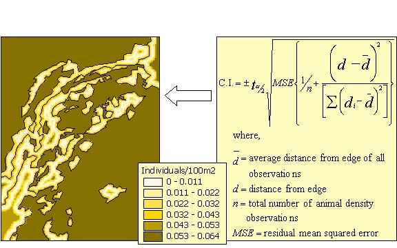
If only two edge distance classes were used, then the ōedgeö and ōinteriorö densities can be entered directly into the EAM, which will assume a linear function. If more distance classes were established, then non-linear or polynomial regression techniques can be used to fit a more complex, continuous function if the data indicate that the relationship is not linear. If a complex function is determined to more accurately portray the edge function, then any non-linear or polynomial formula can be entered into the EAM. For linear functions, a formula for calculating confidence intervals is shown in Figure 9. We are currently researching tractable methods of estimating confidence intervals for non-linear formulas.
The EAM requires the user to input a digital habitat map in polygon shapefile or grid format (Esri, Redlands, CA). In this example, we started with a classified Thematic Mapper Simulator image provided by the Semi-Arid Land-Surface-Atmosphere Program. We clipped a 40 ha riparian area (Figure 4) and used ERDAS Imagine (ERDAS, Inc., Atlanta, Georgia) to eliminate patches less than approximately 300 m2 to create a habitat grid with a minimum mapping unit more appropriate for the modeled edge effects.
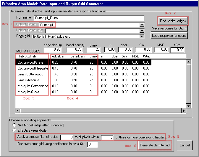
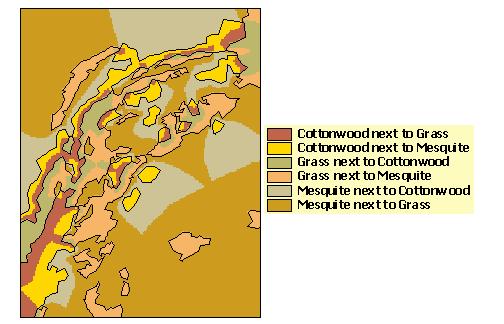
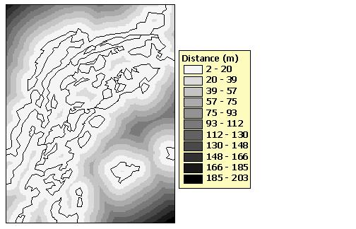
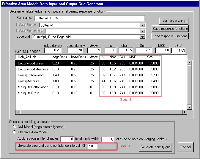
The EAM ArcView extension adds a menu (called "EAM") to the menu bar of the View graphical user interface (GUI). The first EAM menu item opens the dialog box shown in Figure 5, which allows access to most of the major functions of the model. In order to run the model, the user selects a habitat map in the current View with the "Habitat theme" drop down box (Figure 5 - box 1). The user then hits the "Find habitat edges" (Figure 5 - box 2) button and the model identifies all edge combinations (Figure 5 - box 3) present in the study landscape. For example, "Cottonwood|Grass" refers to cottonwood habitat in proximity to grassland. The model accomplishes this by combining the original habitat grid (Figure 4) with a grid derived from it of adjacent habitat classes to create a map showing the unique edge habitats (Figure 6). The edge habitat grid is a classification of the locations over which the model will apply each animal density function. The habitat grid is also used to create a distance to edge grid (Figure 7) to supply distance values for the density functions.
The user must input information on animal edge responses for each species and habitat type used in the model. For this example, we used hypothetical butterfly data that shows consistent edge responses for each habitat type in our study area (Figure 3). Note that our hypothetical butterfly avoids both grassland and mesquite habitat adjacent to cottonwood and exploits grassland next to either cottonwood or mesquite. Also, it shows no edge response in mesquite adjacent to either cottonwood or grassland habitats.
In our example, all animal density response functions are linear and can be added to the "Habitat Edges" list box by entering the EdgeDens (animal density at habitat boundary), BasalDens (animal density in interior habitat), and dmax (the distance of maximum edge response) parameters for each edge type (Figure 5 - box 4).2 Non-linear response functions can be entered via the calculator dialog box accessed by double-clicking any edge type (e.g., Cottonwood|Grass). The model will apply the non-linear function to edge areas until the distance of maximum edge response (dmax) value in the "HABITAT EDGES" table is reached.
When the user has finished entering density response functions, they have the choice of running the null model, which ignores edge effects, or the Effective Area Model, which applies the user-input animal density functions to the landscape. A comparison between the two can be used to highlight the effect of incorporating edge response data. The user also has the option of applying a median filter composed of a moving circular neighborhood to the initial density grid values to estimate local effects of converging habitats (Figure 5 - box 5). This option is not used in this example.
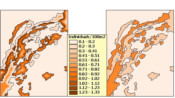
The "Generate density grid" button (Figure 5 - box 6) applies the animal density response functions to their respective edge habitats and distances from edge to form a grid of animal density values (Figure 8). Note the fine-scale patterns added by incorporating edge effects compared to the density grid generated when edge effects are ignored (null model). By selecting the second menu item from the EAM menu, tabular output from the model can also be generated containing descriptive statistics on habitat area, animal density, and population size, including total predicted population for each habitat type within the landscape of interest.
The main goal of our spatial modeling approach is to improve methods for predicting animal abundance and distribution by incorporating empirical data on animal responses at habitat boundaries. To be an improvement, the model should offer both a more powerful estimate of current field conditions and more powerful predictions involving future habitat scenarios. Our goal is not to accurately predict animal density (or any other variable that changes with distance from edges) in any one location at any one point in time. As explained in the section on model validation, we are assessing the ability of the EAM to come closer than the null model to estimating relative animal distributions found in the field. In addition, we are developing uncertainty analysis tools for the user to assess whether predictions made when edge effects are included are significantly different from predictions made assuming constant animal distributions in each habitat.
The main sources of uncertainty in EAM outputs can be divided into two major categories: spatial errors and empirical estimation errors.3 Spatial errors are introduced primarily via the habitat map and empirical estimation errors from the animal density response functions. We are working on several methods to assess the contribution of these errors to model results. For example, we have conducted sensitivity analyses on spatial error and have added an option to the model to calculate the confidence interval associated with edge and interior habitat predictions.
The "natural" or ecological variation in animal density not captured by the regression equations used in our model is due to variables extraneous to distance to edge, some of which may best be modeled as random variables. Extraneous variables include heterogeneous habitat, such as, individual trees or canopy gaps, occurring within what is considered homogeneous habitat during field data collection. The influence of roads, power lines, weather patterns, other species, and numerous other sources, can also influence animal densities.
The EAM currently contains an option to estimate empirical uncertainty by calculating the confidence interval4 for each pixel in the animal density grid using the standard formula shown in Figure 9 (Ott 1993). The user can choose this option by specifying a confidence interval (Figure 10 - box 1) and five regression parameters (n, dbar, Sxx, MSE, and tstat) for each edge type in the Habitat Edges table (Figure 10 - box 2). These parameters are commonly provided by most statistical software packages that support regression analyses.5 This option is currently available only for linear density functions, however we are working on techniques to add the same functionality to the model for non-linear equations.
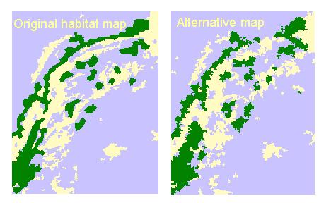
Spatial errors in the habitat map, such as misclassifications of habitat types and positional errors, are translated to the model predictions. We are collaborating with Tony King at Oak Ridge National Laboratory (Oak Ridge, Tennessee) to assess the contribution of spatial error to EAM results. King's group generated ten alternative maps designed to capture the range in spatial error in the original habitat map (Figure 11). We ran our model using these alternative maps to create a probability distribution of possible outcomes.
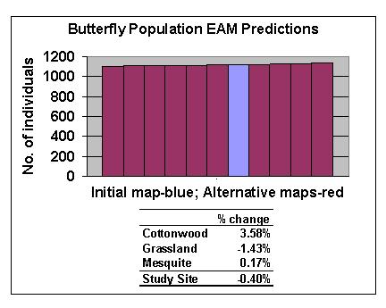
Preliminary results show that the model is not sensitive to spatial error for the species and site tested. The differences in population estimates between the initial and the average of the alternative habitat maps are less than 4% for the entire site and for any one habitat (Figure 12). This is in agreement with other work done in this area (King, pers. comm.). However, investigations are in progress to make more general conclusions regarding the contribution of spatial error to EAM results.
For two of the three habitat classes there were significant differences between the null model and the EAM (Figure 13). Error bars indicate the 90% confidence intervals for the population estimates derived from the error grid for the EAM (Figure 9) and the null model (error grid not shown). The most striking differences between the two models were evident for the grassland habitat because the butterfly increases in density as it approaches cottonwood and mesquite from grassland. This edge effect is not captured by the null model, which overestimates the number of butterflies in cottonwood habitat and underestimates them in grasslands. The EAM predicts that a small percentage of the study area (grassland habitat boundaries) has high density. Since a loss of a small percentage of this habitat could result in a large change in total numbers, this prediction could have important management implications.
Butterfly population predictions for the entire study site do not differ between the EAM and null models due to: 1) the large uncertainty in animal density in the mesquite interior habitat and, 2) the fact that there is no edge effect in mesquite, and, 3) the canceling out of population changes at habitat boundaries since our hypothetical butterfly exploits some edges and avoids others. In this example, error in animal density values has the highest impact in mesquite. If this differentiation is important to the user, they can use the EAM as an aid in assessing where additional field data should be collected, in this case ¢ interior mesquite.
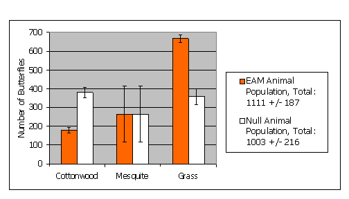
At the three spatial scales discussed in this example, there is no difference between EAM and null predictions at the landscape (study site) scale, large differences at the habitat scale, and even larger differences at the sub-patch and individual pixel scales. Even though the EAM and null population predictions for the overall study site are similar, the models predict striking differences in spatial distribution between habitats and within individual patches, which would have profound implications if landscape structure shifted. In addition, as we analyze model results for multiple species, we will likely see community shifts as animals which primarily exhibit edge avoiding or edge exploiting behavior partition the landscape.
Our goal is to create an easy-to-use predictive model that will be used by managers to make more informed conservation decisions. This model can be used to test the impact of different alternative future land configurations or restoration plans on the ecological community. Of course, the model is only useful if it does a better job of predicting the structure of the ecological community than a null model that doesn't include edge responses.
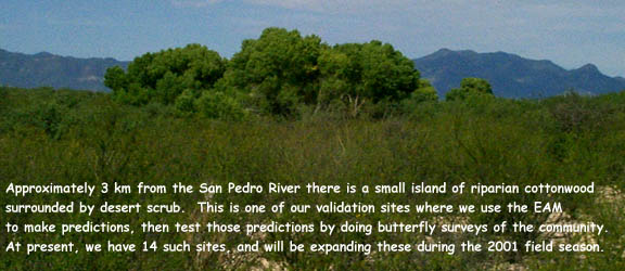
In order to test the ability of the EAM to improve over null models, we are establishing validation sites within and around the San Pedro River. These sites are small, riparian fragments (Figure 14) where we will use the EAM to make predictions about the structure of the butterfly community. We will then perform surveys so that we can compare the actual community to the predictions of the EAM and the null models. We will do this by comparing species rankings or using ordination techniques. If these validation efforts show the EAM to be an improvement over the null model, then we will use the EAM to compare the consequences of different future realizations of the San Pedro habitat based on various land and water-use scenarios. The future realizations of the San Pedro habitat will be created in collaboration with scientists working on the impacts of hydrology and land use on the San Pedro River.
Preliminary model outputs confirm that the responses of animal species to habitat edges may exert profound influence on their distribution in heterogeneous landscapes, and they suggest that the EAM may be a useful tool for guiding habitat management. Ongoing field work will permit more robust parameter estimation and provide field data for testing model predictions. Refinements of the EAM will provide protocols for the characterization of edge responses and address the possible links with life history characteristics, patch size, and other factors associated with heterogeneous landscapes.
To request the current version of the EAM and user manual, see instructions on the EAM web site.
We would like to thank the other members of the Effective Area Model team for their contributions to the design of the model: L. Arriana Brand, James Battin, and Barry R. Noon. The project is funded by the Strategic Environmental Research and Development Program (SERDP Project CS-1100), initiated in spring, 1998.
1. For passerine birds, studies have indicated that edge effects can fall in the 100 to 200 m range (Sisk et al. 2000).
2. The remaining parameters in the list box (n, dbar, Sxx, MSE, and tStat) are discussed in the "Empirical Estimation Error" section of this paper.
3. This presumes that the user minimizes errors in running the model, such as specifying an appropriate pixel size and minimum mapping unit given the species and habitat characteristics modeled.
4. The model actually calculates the upper half of the confidence interval - the difference between the predicted value of animal density and the upper bound of the confidence interval set by the user. We did this so that values from the resulting error grid could be used directly to determine the magnitude of the error bars in the EAM results chart (Figure 13). However, note that because the lower confidence bound could extend below zero at some edge distances in other examples, care must be taken when using the error grid to calculate the lower error bar (e.g., the lower bound of a 90% confidence interval of total population in the study site). We may automate the calculation of unsymmetrical confidence intervals in future EAM releases.
5. The alpha chosen determines both the confidence interval (100[1-alpha]%) and the t-value.
Forman, R.T.T., Godron M. 1988. Landscape Ecology. John Wiley & Sons, New York.
King A. 2000. Oak Ridge National Laboratory, Oak Ridge, TN, Personal Communication.
Naiman, R.J., DeCamps H., and Pollock M. 1993. The role of riparian corridors in maintaining regional biodiversity. Ecological Applications 3: 209-212.
Ott R.L., An Introduction to Statistical Methods and Data Analysis, Fourth ed., Belmont: Duxbury Press, 1993.
Robinson S.K., Thompson III F.R., Donovan T.M., Whitehead D.R., Faaborg J. 1995. Regional forest fragmentation and the nesting success of migratory birds. Science 267:1987-90.
Saunders D.A., Hobbs R.J., Margules C.R. 1991. Biological consequences of ecosystem fragmentation: a review. Conservation Biology 5:18-32.
Sisk T.D., Margules C.R. 1993. Habitat edges and restoration: methods for quantifying edge effects and predicting the results of restoration efforts. In: Saunders D.A., Hobbs R.J., Ehrlich P.R., editors. Nature conservation 3: reconstruction of fragmented ecosystems. Sydney, Australia: Surrey Beatty & Sons. p 57-69.
Sisk T.D., Haddad N., Ehrlich P.R. 1997. Bird assemblages in patchy woodlands: modeling the effects of edge and matrix habitats. Ecological Applications 7 (4):1170-80.
Sisk T.D., Noon B.R., Hampton H.M. 2000. Estimating the effective area of habitat patches in heterogeneous landscapes in J. M. Scott and P. Heglund, eds. Predicting Species Occurrences. Island Press, Covelo.
Stromberg, J.C. 1998. Dynamics of Fremont cottonwood (Populus freemontii) and saltcedar (Tamarix chinensis) populations along the San Pedro River, Arizona. Journal of Arid EnvironmentsĀ40: 133-155.
Stromberg, J.C., Tiller R., and Richter B. 1996. Effects of groundwater decline on riparian vegetation of semiarid regions: The San Pedro, Arizona. Ecological Applications 6:113-131.
Whitcomb R.F., Robbins C.S., Lynch J.F., Whitcomb B.L., Klimkiewicz M.K., Bystrak D. 1981. Effects of forest fragmentation on avifauna of the eastern deciduous forest. In: Burgess R.L., Sharpe B.M., editors. Forest island dynamics in man-dominated landscapes. New York: Springer-Verlag. p 125-206.
Wiens J.A. 1995. Habitat fragmentation: island v landscape perspective on bird conservation. Ibis 137:S97-S104.