James F. Poage, Ph.D.1, Nancy J. Marth, M.S.1,
David C. Goodman, M.D., M.S.1, Stephen Mick, Ph.D.2,
Chiang-Hua Chang, M.S.1, James Dykes, Ph.D.1,
and David M. Bott, Ph.D.1
Abstract
The goal of the Primary Service Area (PCSA) Project is to provide information about primary care resources and populations within small, standardized areas that reflect patient utilization patterns. The PCSA project is the first of its kind to: 1) define primary care service areas throughout the U.S. using standardized methods, 2) encompass actual patterns of primary care use between patients and providers derived from uniform nationwide Medicare claims data, 3) measure nationwide travel costs between populations and their nearest health care providers, and 4) provide data access to a wide range of users, from the novice to the sophisticated, using Geographic Information Systems (GIS) and the Internet.
Introduction
Overview. The purpose of the PCSA project is to define and develop small, standardized geographic units for the entire nation that delineate the actual delivery of primary care clinical services. The need for a system that defines and describes the geographic boundaries of primary care is widely recognized among health care policy makers and analysts. To date, the United States has no such standardized method. Further, there is no primary care service area definition system that is linked to a national database of pertinent health care resources, population descriptors, health care need measures, or utilization statistics that depicts exactly where, how, and how much primary care is delivered to the population. A goal of the PCSA project is to produce just such a system.
Once such a system is developed, validated, and made widely accessible to interested users, it should enhance the ability of health workforce policy makers and analysts to answer a range of important questions. Which geographic locales are demonstrably underserved and to what extent? What characterizes the population of underserved geographic locales? How do such geographic locales correspond to other definitions of underservice? Public and private efforts to promote improved access to primary care should benefit by having a proven method that defines the geographic areas of actual use.
In order to achieve the goals of the PCSA project, the team used GIS and the Internet to develop a comprehensive national database of primary care service areas that is easy to revise and updated. Furthermore, this national database will soon be accessible to a broad array of potential users with diverse objectives. Users will be able to access the maps and data through an Internet web site running Esri’s ArcIMS. In addition, registered users will be allowed to download health care attributes with their associated boundary files to use in health research and analysis.
As of June 2001, 6,102 PCSAs have been defined in the U.S and are comprised of one or more ZIP Codes. In addition, the project team has developed a master database of geographic, demographic, and health care variables that may be joined to various geographic boundary shapefiles. These boundary files were obtained from Geographic Data Technology (GDT) and include ZIP Code, Minor Civil Divisions (MCDs), Census Tracts, County, and State boundary files. Files from the Health Care Financing Administration (HCFA) were used to define the PCSAs and were further analyzed to describe Medicare beneficiaries medical care utilization. These files include: Medicare Part B file (a 5% sample), Medicare Denominator files, Medicare Outpatient Files, Supplemental Part B files, Medicare Provider of Services file, the AMA Physician and AOA Osteopath files, and. Demographic data was provided by Claritas and was derived from the 1990 U.S. Census with updates to reflect demographics for 1999 at particular geographic levels. Claritas also provided updated Congressional District (CD) and Metropolitan Statistical Area (MSA) boundary files. All the data used to create the master database and for user access via the web site will be licensed in one way or another, for both the original data and for all derivative products.
PCSA Delineation (‘Crude’ Assignments)
Several statistical processes were performed before importation into the GIS: 1) the Medicare Denominator file was used to identify eligible beneficiaries, 2) all claims record for eligible beneficiaries were combined from various sources into a single data set, 3) only claims representing primary care were identified and selected, and 4) ‘crude’ PCSA assignments for each ZIP Code were created based on a patient origin matrix derived from the combined data set.
Assignments based on utilization. With this last step, the process began with the identification of provider ZIP Codes and the calculation of the proportion of each beneficiary’s utilization to each provider ZIP Code. Crude PCSAs are created by assigning each beneficiary (or population) ZIP Code to the provider ZIP Code providing the most primary care utilization for that specific beneficiary ZIP Code.
ZIP Codes with at least one Medicare provider submitting a minimum of 50 weighted Medicare primary care claims were coined ‘provider ZIP Codes. This value was selected to eliminate provider ZIP Codes from data entry errors or extreme part-time provision of care, such as a clinic closing the first week of the data year. ZIP Codes with at least one Medicare beneficiary resident were termed ‘population ZIP Codes.’ Beneficiary utilization was measured in numbers of weighted claims based on the beneficiary sample size at the ZIP Code level of the origin data set.
Each beneficiary’s claims were analyzed to identify the total number of weighted claims for that beneficiary and the total number of unique provider ZIP Codes in which services for that beneficiary were obtained. In order to control for very sick patients with high levels of utilization, each beneficiary was assigned a preference ‘vote’ of 1. The proportion of a beneficiary’s total weighted claims located within a particular provider ZIP Code is termed a ‘preference fraction.’ The sum of these preference fractions for a single beneficiary equaled 1. For example, a beneficiary receiving three services in one provider ZIP Code and two services in another provider ZIP Code would have a preference fraction of 0.6 for the first provider ZIP Code and a preference fraction of 0.4 for the second provider ZIP Code. The sum of that beneficiary’s preference fractions must always equal 1.0.
The crude PCSA file was derived from the patient origin matrix and contains a row for each population ZIP Code with the preliminary PCSA assignment and additional columns of other provider ZIP Codes and their associated preference fraction sums. Other columns or fields of demographic data were added to aid the geographic analyst in applying criteria for final PCSA assignments.
PCSA Reassignment with GIS
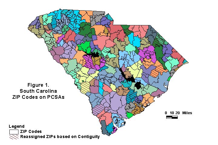
Reassignment Sequence. The PCSA reassignment process was characterized at two levels by reassigning both population ZIP Code polygons and entire PCSAs to other provider ZIP Codes or PCSAs instead of their original, crude assignments. This process was based on a series of sequential checks, first at the population ZIP Code level, then at the PCSA level. Population ZIP Codes were reassigned if 1) provider ZIP Codes had less than 50 Medicare claim visits (as described above) and 2) the PCSA was discontiguous. Subsequent reassignments at the PCSA level occurred if 1) the entire PCSA did not retain the plurality of its preference fractions, 2) the PCSA had a preference index <= 0.030, and 3) the PCSA had a total census population of less than or equal to 1,000.
Most PCSA reassignments were based on contiguity (Figure 1). The goal of ensuring contiguity for each PCSA was to create units that were easily related to other geographic areas such as census tracts, MSAs, counties, hospital service areas, hospital referral regions, and states. The crude assignment file was joined to ZIP Code boundaries and converted to a shapefile. The contiguity step involved reassigning population ZIP Code polygons that were not contiguous or adjacent to the other ZIP Code polygons that comprised a PCSA. Contiguity required the geographic analyst to visually examine the crude PCSA assignment polygons and manually reassign population ZIP Codes to ensure a ‘new’ contiguous PCSA (‘donut’ PCSAs--small PCSAs within a larger PCSA were allowed). Reassignment for both contiguity and plurality involved knowledge of the statistics provided in the crude PCSA file to adequately reassign the ZIP Codes or PCSAs. Additional geographic shapefiles such as roads, geocoded rural health centers (RHCs) and federally qualified health centers (FQHCs), and ZIP Code centroids were used to help refine the reassignment methodology.
After processing for contiguity, the ZIP Code reassignments were exported from the GIS and sent to the statistical analyst for recalculation of the PCSA level utilization and demographic statistics. The next sequential check would ensue. At each reassignment stage, a field would be added to the crude assignment file, reflecting a code of how and why a particular record was reassigned. This allows an assignment trace on each population ZIP Code and PCSA in the database.
Pilot States. The PCSA delineation and reassignment process was initially applied to nine pilot states: Maine, New Hampshire, Vermont, South Carolina, Florida, Michigan, Kansas, Missouri, and Utah. These states were chosen to test and modify project methods before applying them to the other 41 states. The states also represent diverse populations, geography, race, ethnicity, and health status.
The project team needed to enlist the experience of the pilot states’ Primary Care Offices (PCOs) and Primary Care Associations (PCAs), to evaluate the project methodology and increase the usefulness of the PCSA database. Therefore, individual state meetings were held where project processes were explained and summary statistical tables and PCSA maps were presented. Each meeting contributed insight and a further understanding of state policy concerns, data needs, and computing capabilities.
Travel Time Task
Background. Geographic accessibility to health care resources has become an important aspect of statewide health care planning. Various statewide studies have been conducted to evaluated patient travel time and distance to nearest medical facilities. Traditionally, travel distance has taken precedence in determining the geographic accessibility of patient to medical care resources (Bosanac et al, 1976). However, due to further developments of data capture in the transportation planning field, additional factors such as landscape variability, traffic congestion and patterns, can be used to determine travel time, a more accurate measurement of accessibility. From previous studies, a 30-minute travel time designation has become a standard in which to designate medical resources as either accessible or inaccessible to health care populations. With this standard, along with socioeconomic data, populations can be characterized and their health care needs assessed. Those outside the 30-minute standard may be eligible to apply for assignment of National Health Service Corps personnel, if designated as health manpower shortage areas (Federal Register, 1980).
Health care accessibility studies have usually been constrained to regional or local geographic areas, partly due to specific need and readily available local data sets. Since a primary goal of the PCSA project was to create localized areas of primary care resources, an idea surfaced to apply a travel time definition to the project, as well. Hence, the PCSA travel time study aims to characterize geographic accessibility on a national level, using ZIP Code level data to represent patient populations and physician locations in order to identify geographic areas as possible health manpower shortage areas.
Software and data. Since project tasks were previously accomplished using Esri products such as ArcView for the PCSA creation process, Network Analyst was chosen to perform our travel cost functions. ArcInfo’s NETWORK module was considered but the Geographic Analyst was more versed in ArcView and Avenue, than ArcInfo Workstation, NETWORK, and AML. ArcInfo 8.0.2 Desktop was an option but the processing performance on our computers was substandard to that of Workstation ArcInfo or ArcView. ArcLogistics and RouteMAP were considered but neither allows for batch processing between two large point files or addresses a ‘Find Closest Facilities’ type of problem.
The process of identifying an adequate, affordable network data set was daunting. Road data is plentiful, but for routing problems, impedance such as speed limit, time cost per line segment, one-way, over- and under-pass, and turn restriction information is needed. Impedance and road detail was needed down to at least the county level. Esri provides some impedance attributes with the National Highway Planning Network (NHPN) road data accompanying the Network Analyst extension but the level of detail was not adequate. Road data existed from a previous Geographic Data Technology (GDT) purchase but the data did not include any impedance. After researching costs with data vendors, GDT’s Dynamap Highways/Routing product was purchased for our network data set. Street-level data detail was preferable but too costly. Esri’s StreetMap product at that time did not include some needed routing impedance attributes.
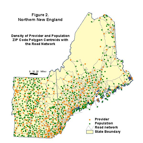
Methodology. PCSAs have been derived from ZIP Code level data and not actual addresses, due to the mandatory suppression of this Medicare data below the ZIP Code level. Hence, geocoding patient addresses was not an option to represent exact locations in our travel study. In order to calculate travel time between patients and physicians (or providers), their geographic locations were approximated by ZIP Code level service centroids. ZIP Code service centroids were used to represent the bulk of ZIP Code populations and the locational likelihood of provider facilities. The goal was to calculate the travel time and subsequent mileage along a road network from each ZIP Code polygon service centroid (origin), representing the population of health care consumers, to the nearest two ZIP Code polygon service centroids (destination), representing the provider facilities.
Origin and destination ArcView shapefiles were subset from nationwide ZIP Code centroid shapefiles. There were approximately 30,000 ZIP Code polygon centroids and 15,000 physician or provider centroids. Provider ZIP Codes were defined as those physicians with a minimum of 50 Medicare visits or claims within the 1996-97 Medicare data.
Once the network data was obtained, road speed assignments were reviewed. The existing speeds assigned to each road segment within a particular road class (interstates, state highways, etc.) were acceptable but did not reflect the urban and rural character of the network. Therefore, for each road class, speeds were redefined for the entire network based on their proximity to Metropolitan Statistical Areas (MSAs) and urban areas. After reviewing outside sources to locate a nationwide standard of road-speed assignments (there is none), our project team decided upon a set of nationwide, average urban and rural speeds for each road class. Through a series of geoprocesses, road segments were assigned an ‘R’ or ‘U’ based on whether or not they were contained within an MSA or urban polygon. Urban roads were collectively assigned slightly lower speeds than rural roads. The road segment cost in minutes was subsequently recalculated to reflect the new speeds for each road segment in the network.
Since the Network Analyst interface only accommodates interactive origin to destination matches in a ‘Find Closest Facility’ problem, it was necessary to edit an existing ‘Find Closest Facility’ sample script to run in conjunction with NA. Edits were made to a) perform a batch process to locate the nearest two destinations from each origin along a road network and create a graphic path between them, b) set the network search tolerance to locate centroids not intersecting the road network, c) calculate the distance of each path, and d) add a progress meter and other small, miscellaneous additions.
A sample region, northern New England (Figure 2), was processed and the output was compared to other sources for evaluation. These checks included the comparison of ‘likelihood of path’ chosen by a research associate and his choice of fastest route(s) and the actual distance measurements along roads in state gazetteers (atlases) of those routes to the program output. Additional checks were made comparing the travel cost in minutes, path taken, and distance output with an outside, interactive mapping software package, DeLorme’s MapItä software.
Because of the time-consuming processing and extensive memory needed to run the entire nation, the centroid and road network files were processed on a regional basis, with overlapping areas to account for travel time paths crossing state borders. The output files were then appended and edited to include only the two least cost paths in minutes between each origin and destination pair.
Present task status. While travel time computations will be performed for the entire U.S., we have completed northern New England calculations between each population centroid and its nearest two provider centroids. As with the PCSA reassignment process, a portion of the country was taken as a test site in order to refine certain methods before they are applied to the remainder of the data. The tasks mentioned below are being addressed at this time for northern New England.
As previously mentioned, the travel time script incorporates a network tolerance for centroids that do not intersect a road. The travel time path begins at the closest point on the road to that centroid. The next steps are to create additional code or use an ArcView extension to calculate the distance from each centroid to the nearest road, specify an average speed associated with that distance, and calculate the additional travel time centroid to road cost in minutes and miles and add those values to the existing path cost in minutes and miles.
Also, centroids outside the network search tolerance that were not included in the original calculation need to be identified, the tolerance extended, and the script rerun to calculated their travel time path in minutes and mileage.
To minimize distortion in the travel time path distance and the centroid to road distance calculation, it may be preferable to divide these regions into smaller areas and apply a different projection before the calculation is made. The largest travel time path distance is a matter of a few hundred miles, while the largest centroid to road distance is approximately twenty miles. Both are relatively small values versus cross-country distances, so the projection chosen is somewhat dependent on scale of the data and requires different consideration.
Of course, before any data set is considered final, statistical checks are necessary to validate the output. These statistical checks will include examining frequency distributions, ratios of speed to distance, and standard deviation calculations between the longest path straight line distance and the travel cost path distance.
Dissemination of Project Data
Hardware and Software. The web site prototype system is based on two NT 4.0 servers, one running the web services and another running ArcIMS. The server handling the web runs Apache Server Side Include (SSI) software for the web engine. It allows dynamically created additions to an HTML page. The Apache web server will serve the PCSA project web pages and help files, allow data downloads, contain the master database to allow creation of new data files, and use HTML to link to the ArcIMS server.
The web site system was placed on two different servers for performance reasons. From project experience, the ArcIMS server requires its own box because of the heavy load it places on the hardware. By placing the Apache web server onto a separate box, the load that the beginning users place on the ArcIMS server will not interfere with the intermediate and advanced users downloading data and looking at help files. The project team estimates that this configuration will support 2,000 users, the benchmark initial number of PCSA users.
In contrast, the project team found that the ArcIMS server places a considerable load on the hardware on which it is running. Each ArcIMS user request loads the CPU and I/O system on the hardware to 100% for up to several seconds. Each request requires retrieval of maps and data, then the maps and data must be combined together, clipped, and sent to the user. Once this operation is complete, the server pauses and is ready for another user. Testing shows that 10 "simultaneous" users is the most the ArcIMS server can handle. With 10 users, during one user’s pauses, another users can request information from the server. With 10 or fewer users, the requests tend not to overlap. For more than 10 users, the requests tend to overlap more and the response time from the server gets considerably longer. Although the server can handle more than 10 simultaneous users, system performance becomes unacceptably slow.
Delivery Overview. The planned data delivery system allows users of all experience levels to have access to the PCSA data. The system is based on a web site which allows users to access interactive maps through ArcIMS, download GIS ArcView project files for analysis via an ftp site, or download the entire master database (subject to appropriate suppression) and corresponding shapefiles for analysis with other software. The system uses a static delivery model for the data; this means that all maps, projects, and data will be created by the project team and placed on the web site for subsequent download by the users. The data to be downloaded are compressed by Eagle Information Mapping’s Viewpoint Transporterä program for faster transmission. The Viewpoint Retrieverä software that expands the project file and saves the download on the client side is available free of charge on their Internet web site.
Users will gain experience as they work with the
web site and data. Although, the full features of the PCSA project are
available only to those users who can use a GIS system, tutorials and help
files will be provided to ease their transition into GIS software. Table
1 summarizes the user levels, the computer experience users are expected
to have, and what they will be able to do. Beginning users will have access
to the PCSA data through web-based interactive maps. Intermediate users
will be able to download ArcView project files via ftp for custom analyses
that include adding local data. For the advanced users, data, shapefiles,
and sufficient documentation will be provided so that they can have full
flexibility in performing analyses.
|
|
|
|
| Beginner | Use a web browser. Familiar with at least one spreadsheet and word processor program. | Use interactive maps to look at primary care in his or her area. Download data into reports or spreadsheets. |
| Intermediate | Some experience with GIS software. Has used a database to query data. | Link local data with PCSA project files for custom analyses. Create custom maps. |
| Advanced | Very familiar with GIS software. Knows how to read in raw data and link data to shape files. | Perform analyses with all PCSA data. Load new data. Create custom maps and data. |
Table 1. Levels, computer experience, and tasks performed by PCSA users.
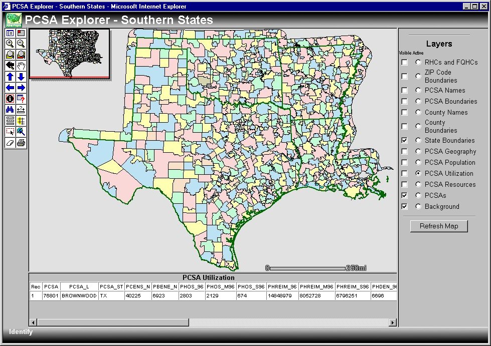
In order to make the PCSA data as useful as possible, the data will be customized to the user level. The interactive maps will focus mainly on PCSA and ZIP Code-level data and consist of the most important provider, population, and utilization characteristics. These maps will be created for regions of the country, instead of the entire country, to allow users to more quickly access data and maps (Figure 3). The ArcView project files for intermediate users will again be focused on regions of the country but will also include information from additional geographic levels such as state, county and census tracts. The project files will also include a wider variety of variables than those found in the interactive maps. These files will allow a user to load the data and shapefiles easily into a GIS system. The GIS system will also let them combine the PCSA data with local data to perform custom analyses. Advanced users will probably want as much flexibility as possible; therefore they will have access to the entire master database (with suppression), shapefiles, and full documentation. The suppressed database will have many more attributes in it than are presented through ArcIMS or are included in ArcView project files. Each level of user will have access to the data and variables that are most useful to them.
Users will be required to register before they can access either the interactive map servers or data. Registration is necessary to comply with licensing restrictions on the data, and will enable a way to update users on new data or changes to existing data. Users will fill in a form requesting, among other things, a valid e-mail address. Once the form is processed, the user will receive an e-mail back with a registration key.
Figure 3. Southcentral U.S. PCSA region
served by ArcIMS
Design Considerations. The design process began with the idea that ArcIMS could serve both beginning and intermediate users through a web browser, and that the intermediate users could add local data through their web browser. While this is technically possible with ArcIMS, the Java versions require the user to install ArcIMS Viewer, ArcExplorer, and a Java Plug-in. Furthermore, the Java version requires a high bandwidth that would be unavailable to many users. Instead we have settled on the ArcIMS HTML version for beginners, a local GIS (primarily ArcView), for the intermediates, and full data files for the advanced users.
Working with the pilot states, many of the PCOs and PCAs already had one or more people on their staffs working with GIS systems including Esri, MapInfo, and lesser-known products. Overall, the level of GIS expertise with these products was very low. ArcView was the most commonly used GIS, and HRSA has elected to use ERSI products as its GIS standard. The project team decided to create ArcView-based project files to simplify the process of using PCSA data for intermediate users. By supplying project files and providing documentation on how to use them, the state PCOs and PCAs can quickly start using the PCSA data. With the project files as a starting point, GIS users can easily link in their own data.
One final consideration was deciding how to register users. Most web servers supply some method of registering users. Typically, this method allows an unregistered and registered area on the web site. It can also be secure (typically using SSL), or in the clear (passwords are sent through the Internet unencrypted). ArcIMS is different--technically, it is possible to register users specifically for ArcIMS, but then there’s a matter of synchronizing the ArcIMS user database with that for the home web site. Instead, the unregistered users will be allowed to preview our ArcIMS site through a series of screen snapshots presented on the home web site. Users will enter the registered web site through the home site, which will run Apache on a Windows NT server. The "registered" web pages will contain the hyperlinks to the ArcIMS site.
From the perspective of a client, perhaps the most significant change in our web site design since June 2000 has been the elimination of a data browser, such as ArcExplorer, as part of the data dissemination plan. While ArcExplorer does permit clients to create their own maps from shapefiles that they could download, it does not permit the addition of new attributes to those maps from local sources. One must use a product such as ArcView 3.2 to have the ability to edit the data or join new tables to geographic features on a map.
Project Status
Presently, the web site is in place and the regional shapefiles have been joined with demographic and health-related attributes from the master database. The PCSA web site will be ready for access October 2001. It will serve various health care agencies and individuals such as State Departments of Public Health, PCOs, PCAs, Area Health Education Centers (AHECs), state workforce centers, community health centers, Offices of Rural Health Care, and other local, state, and federal agencies for health policy decision-making and research. Recently, it was agreed that HRSA would eventually serve the maps and data from their own ArcIMS site at their building. Nevertheless, additional time will be spent refining the web server and ArcIMS to be as user-friendly and easy to use as possible. The duration of the project will also involve creating and testing project files, updating the documentation of the master database; creating documentation and help files for users; and finishing travel time calculations, checks and corrections.
References
Bosanac, Edward M., M.S., Rosalind C. Parkinson, M.A. and David S. Hall, Ph.D. "Geographic Access to Hospital Care: A 30-Minute Travel Time Standard." Medical Care. 14 (1976): 616-624.
Federal Register. "Criteria for designation of health manpower shortage areas." Federal Register. 45 (1980): 75996-76003.
Poage, James F., PhD. "Natural Market Areas for Primary Care Health Services: How does one determine them? How does one publish the information? Why does one care?." Twentieth Annual Esri International User Conference. CD-ROM. August 2000.
2 Virginia Commonwealth University
Department of Health Administration
1008 East Clay Street
Richmond, VA 23298