Environmental Sensitivity Index maps have been developed to map coastal areas to prepare and respond oil spills. The ESI data represent the wildlife and habitats which are sensitive to spilled oil. Regions are implemented to store, edit and create maps which consist of numerous overlapping polygons and detailed relational database tables. This paper describes the data structure used to store, manipulate and display numerous biological and human-use layers of information.
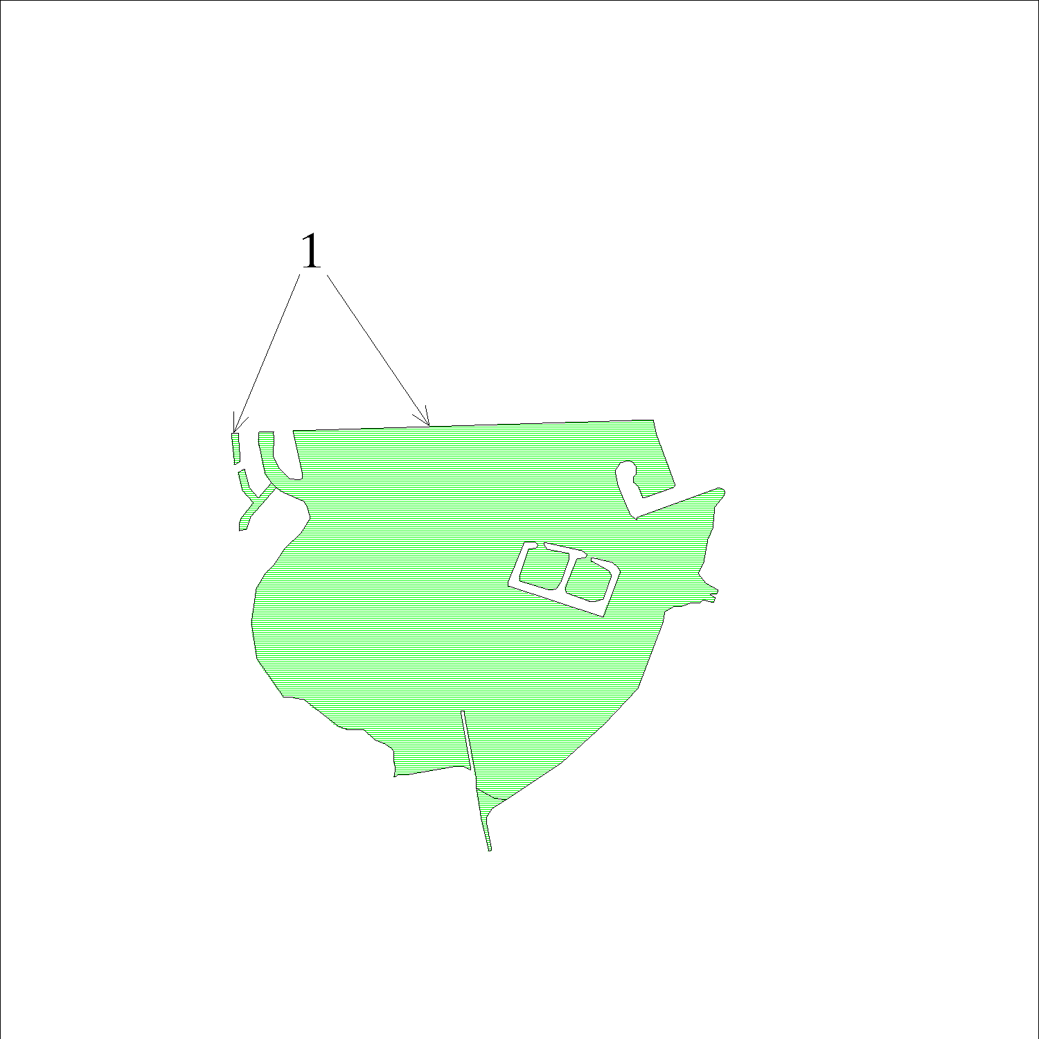
ESI MAPPING
Describe quickly the history of esi mapping.

GIS DATA STRUCTURE FOR ESI MAPPING
	ESI data characterize coastal environments and wildlife by their
sensitivity to spilled oil.  There are three main components to describing
the sensitive features: shoreline habitats, sensitive biological resources,
and human-use resources.  There are many layers of information which are
gathered and either digitized or reformated to match the data structure.
The following coverages comprise an ESI atlas:
	ESI - classified shorelines and habitat polygons
	HYDRO - water and land polygons and linear streams
	INDEX - quad boundary polygons
	MANAGEMENT - managed land regions
	SOCECON - human-use point and line resources
	MAMMALS - terrestrial and marine mammal regions
	BIRDS - bird regions
	NESTS - bird nesting point locations
	FISH - fish regions
	SHELLFISH - mollusc and crustacean species
	REPTILES - reptile regions

ESI Shoreline Geomorphology:
	The ESI coverage contains both linear shoreline geomorphology
as well as polygonal habitats which are marine or tidally influenced.
Each line and polygon feature is classified according to the suscept-
ability of impact to oil spills.  The classification varies by geographic
condition, but generally has the following categories:
	ESI RANK	DEFINITION
	1		Exposed, impermeable vertical substrates
	2		Exposed, impermeable non-vertical substrates
	3		Semi-permeable substrate, low potential for oil
			penetration and burial
	4		Medium permeability, moderate potential for oil
			penetration and burial
	5		Medium-to-high permeability, high potential for
			oil penetration and burial
	6		High permeability, high potential for oil
			penetration and burial
	7		Exposed, flat, permeable substrate
	8		Sheltered impermeable substrate, hard
	9		Sheltered, flat, semi-permeable substrate, soft
	10		Vegetated wetlands

	The classification of shoreline habitats are modified to adapt
to site specific conditions and in many cases the shorelines are ranked
with multiple codes such as 10/2.  Also included in the ESI coverage
is a code to describe the arc feature:
	FEATURE CODE	DEFINITION
	S		Shoreline
	I		Index or map/quad boundary
	H		Hydrography or streams
	P		Pier
	B		Breakwater
	O		Other arcs which form the boundary for ESI
			polygons but are not shoreline.

	To document the digitizing process for ESI classification an
attribute is included with every feature for the source of the data.
The source codes are:
	SOURCE CODE	DEFINITION
	0		Digital data (provider documented in the Meta
			Data Report for each atlas)
	1		Ground truth
	2		Aerial photograph
	3		Digitized from USGS topographic quadrangle
	4		Line approximated to ensure edgematching
	5		Digitized on-screen from scanned USGS quad.

Basemap Coverages:
	The coverage HYDRO contains polygonal water and land features
as well as all tidally influenced linear stream features.  Also included
in this coverage are all annotations which are present in the water
portion of USGS topographic quadrangles as well as many others which
have been identified as important land features.
	The coverage INDEX contains polygons for all 7.5 minute USGS
topographic quadrangles in the atlas.  Each polygon is attributed for
quad name (including date or revised date), the scale at which the map
is produced, the map angle used to rotate the coverage so that north is
truly at the top of the map, and the page size of the map.

Human-Use Coverages:
	The are many human-use (or socio-economic) features which are
important for preparing or responding for oil spills.  These are generally
impacted either economically due to polution, operationally as people
and equipment are brought in to clean up the site or are sensitive human
resources which must be protected.  The following features are mapped in
an ESI atlas:
	FEATURE		DEFINITION
	A2		Access
	A		Airport
	AQ		Aquaculture
	AS		Archaeological Site
	B		State Beach
	BR		Boat Ramp
	CF		Commercial Fishing
	CG		Coast Guard
	CP		Campground
	F2		Factory
	HS		Historical Site
	H		Hoist
	IR		Indian Reservation
	IB		International Border
	LS		Log Storage
	M		Marina
	M2		Mining
	MS		Marine Sanctuary
	NP		National Park
	OF		Oil Facility
	P		Regional or State Park
	PF		Platform
	PL		Pipeline
	RB		Recreational Beach
	RF		Recreational Fishing
	S		Subsistence
	SB		State Border
	V		Village
	WI		Water Intake
	WR		Wildlife Refuge

	Each feature in the SOCECON and MANAGEMENT coverages contains a
unique identifier, termed RARNUM or resource at risk number, which is
linked to an Oracle table which stores items such as the contact person,
the owner of the facility, the phone number and site specific comments
such as the number of slips at a marina.

Biological Coverages:
	Coverages for biological data are developed for each major
element of the ESI atlas.  The coverages include: BIRD, FISH, SHELLFISH,
REPTILE, MAMMAL and PLANT.  For many atlases, bird nesting sites are
also digitized in a NEST coverage with point topology.  The following
subelements are collected for each element:
	ELEMENT			SUBELEMENT
	Marine Mammal		Dolphin, Manatee, Sea Lion, Sea Otter,
				Seal, and Whale
	Terrestrial Mammal	Bear, Deer, Mustelid, Rodent
	Bird			Alcid, Diving Coastal Bird, Gull/Tern,
				Pelagic, Raptor, Shorebird, Wading Bird,
				and Waterfowl
	Fish			Anadromous, Beach Spawner, Kelp Spawner,
				Nursery Area, Reef Fish, and Special
				Concentration
	Shellfish		Abalone, Clam, Conch/Whelk, Mussel, Oyster,
				Scallop, Squid/Octopus, Coral Reef, Crab,
				Lobster, and Shrimp
	Reptile			Alligator/Crocodile, and Sea Turtle

	The release of ArcInfo rev. 7.0.2 enables the biological data,
which is complex, to be topologically stored as regions.  The following
section describes the use of region topology to store the complex
polygons and tabular data.

IMPLEMENTATION OF REGIONS
	The biological data in ESI atlases are complex structures due to
the natural mixture of several species within and across habitat types.
To describe the efficiency of data storage, editting and reproduction
of the complex data a small portion of an area in Southern California
is descrbe for the presence of birds (Figure 1). In this example a discon-
tiguous region is one where multiple, nonadjacent, polygons are grouped
together to form one region.  This method of labeling, or attributing a
database is efficient for data storage and quality control.
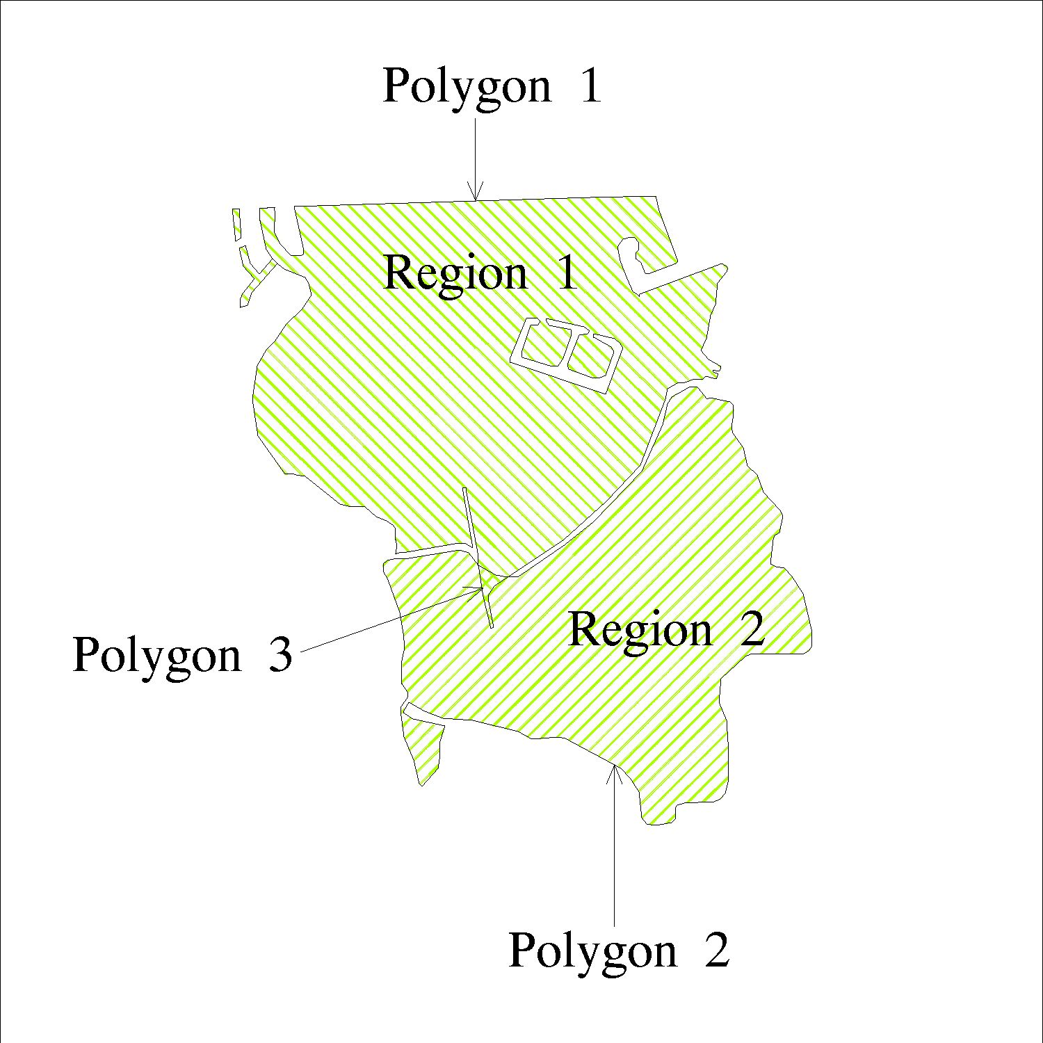
Another type of region is the overlapping region where only two
attributes are entered (Figure 2). For instance, Polygon 1 and Polygon 3
contain the same species and are defined as Region 1 and Polygon 2 and
Polygon 3 contain the same species and are defined as Region 2.  In this
example Polygon 3 is used for both Region 1 and Region 2.
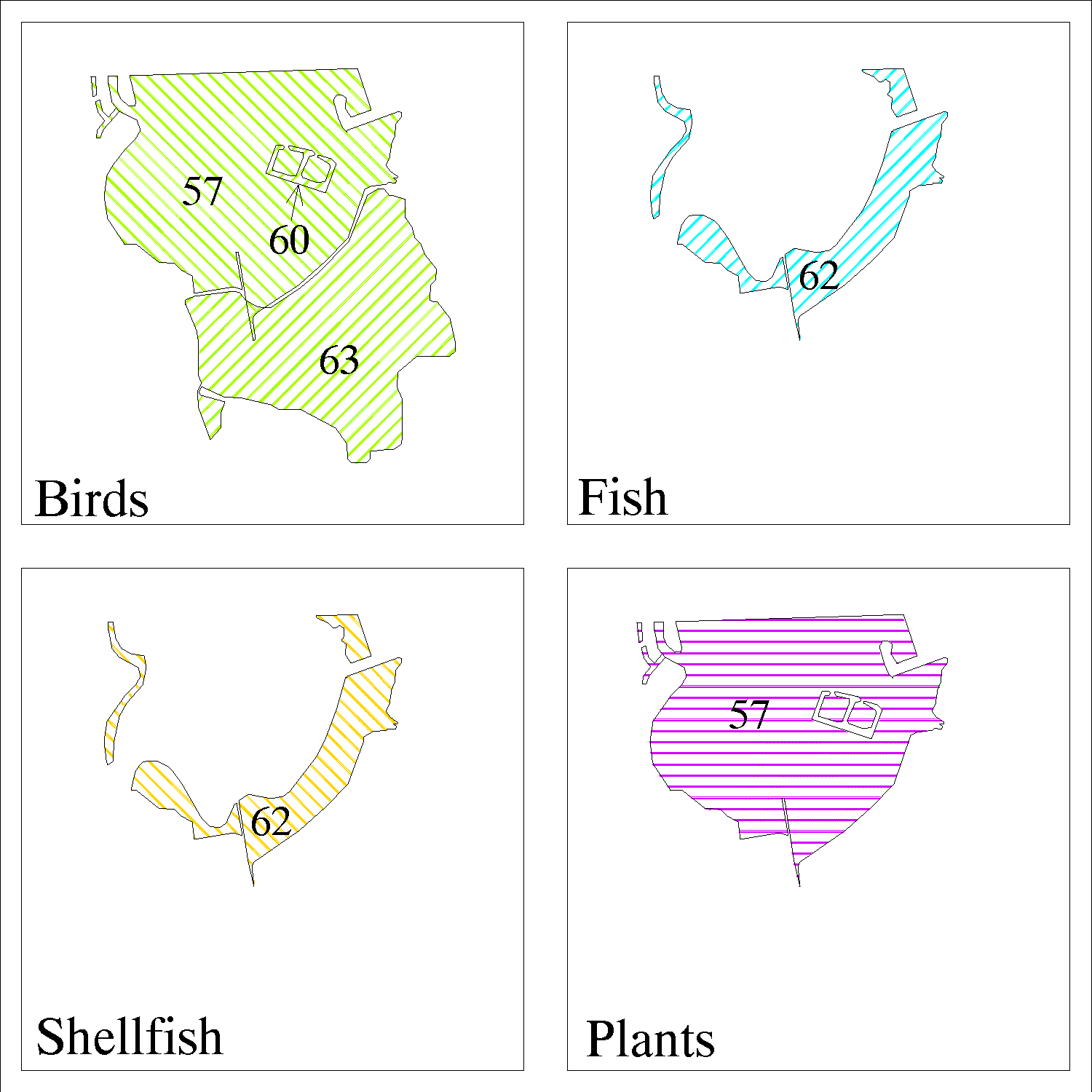
In the ESI database, all biological elements (and therefore species) may
be in geographic combination which is difficult to maintain at the polygon
level, but easier from a data management perspective at the region level
of topology because there is minimal data redundancy.  For example, there
are multiple coverages with the same RARNUMs for birds, fish, shellfish
and plants (Figure 3).  These seperate coverage share many arcs and
polygons and regions.  In this example, unique identifiers (RARNUMs) are
shown for each region and each region may be comprised of one or more
polygons.  Although the elements are stored in seperate coverages, the
linkage of RARNUMs enables the database to remain efficient.  This is
evidenced by Region 57 which is in the BIRDS and PLANTS coverages and
Region 62 which in in the FISH and SHELLFISH coverages.  Another example
of a discontiguous region is RARNUM 62.  In polygon topology the value 62
would be entered for all four polygons in the FISH coverage and also the
four polygons in the SHELLFISH coverage.  This polygon data structure is
redundent, it increases the probability of a data entry error and it limits
the analytical power of the database.
For each RARNUM there is an Oracle Table (BIO_RES) which specifies the
contents of the region.

Table 1. Contents of Oracle table BIO_RES which correspond to Figure 1.
RARNUM	SPECIES	CONCENTRATION	SEASONALITY	EXPERT	ELEMENT
57	85	HIGH		1		58	BIRD
57	118	HIGH		2		58	BIRD
57	270	HIGH		1		58	BIRD
57	1001	HIGH		1		58	BIRD
57	1002	HIGH		1		58	BIRD
57	1003	HIGH		1		58	BIRD
57	1004	HIGH		1		58	BIRD
57	1005	MED		1		58	BIRD
57	1006	HIGH		1		58	BIRD
57	22	LOW		2		55	M_MAMMAL
57	1	HIGH		1		58	PLANT
60	85	HIGH		1		58	BIRD
60	270	HIGH		1		58	BIRD
62	225	HIGH		1		0	FISH
62	24	LOW		1		0	SHELLFISH
62	28	HIGH		1		0	SHELLFISH
62	66	HIGH		1		0	SHELLFISH
63	85	HIGH		1		58	BIRD
63	118	HIGH		1		58	BIRD
63	205	LOW		1		58	BIRD
63	270			1		0	BIRD
63	1001	HIGH		1		58	BIRD
63	1002	HIGH		1		58	BIRD
63	1004	HIGH		1		58	BIRD
63	1006	HIGH		1		58	BIRD

The SPECIES and ELEMENT variables are used to link to the Oracle Table
SPECIES which contains the common and latin names, abbreviation, and the
status for threatened or endangered at the federal or state level.

Table 2. SPECIES list for records in Table 1.
SPECIESELEMENT  SUBELEMENT NAME			GEN_SPE		S_F	T_E
85     BIRD	gull_tern  California least ternSterna antillarum brow. F E
118    BIRD	diving	   Brown pelican        Pelecanus occidentalis  F E
205    BIRD	wading     Light-footed clapper rail,Rallus longirostr.
270    BIRD	shorebird  Western snowy plover Charadrius alexandrinus.
1001   BIRD	gull_tern  Gulls
1002   BIRD	shorebird  Shorebirds
1003   BIRD	waterfowl  Waterfowl
1004   BIRD	wading	   Wading birds
1005   BIRD	raptor	   Raptors
1006   BIRD	diving	   Diving birds
1      PLANT	sav	   Eelgrass		Zostera marina
225    FISH	special	   California halibut	Paralichthys ca.
22     M_MAMMAL sea_lion   California sea lion	Zalophus califo.
66     SHELLFISHclam       California jackknife clam,Tagelus californianus
24     SHELLFISHclam       Gaper clam           Tresus nuttallii
28     SHELLFISHclam       Pacific razor clam   Siliqua patula

The SEASONALITY and EXPERT columns from the BIO_RES table are linked to
other tables which identify the months that species are present and
the activity during those months, such as nesting or laying.  The EXPERTS
table contains a complete meta data reference for contacting specific
places, agencies and personnel in the event of an oil spill.

CONCLUSION
This paper presented a format for organizing polygonal overlapping and
discontiguous polygons as regions.  These regions are linked to multiple
Oracle Tables.  The data structure is efficient, easily edited and has been
implemented to produce map atlases.  Currently, Research Planning Inc. has
produced eleven GIS ESI atlases along the United States coastline and six
atlases will be completed in 1995 using region topology.  The transition
from polygons to regions was almost effortless at the data entry stage;
however, there was quite a learning curve in the aml process of producing
the hard copy maps.  Future goals are to reduce the biological coverages to
just one coverage which will reduce the data redundency even further.
However, we have decided to take gradual steps in the introduction of
regions in order to minimize the length of time learning as well as become
comfortable with the new techniques.

ACKNOWLEDGEMENTS:
I would like to thank Mr. William Holton, the System Administrator at
RPI, for quickly producing the graphics used in the paper.