A method was developed to transfer data from a finite-element ground-water flow model into ARC/ INFO1 and also to transfer data to the model so that the data interpolation, integration, and display capa bilities of ArcInfo could be used. Model-calculated values and data from a program that generated the finite-element mesh were supplied as ASCII files. These data were converted to coverages by loading the files into INFO and manipulating them to produce files in polygon GENERATE format.
Model-node loca tions in the mesh were edited in ARCEDIT to more closely align with geographic features and then were transferred to the model as edited UNGENERATE files. Data from different sources were combined to create an integrated surface represented by a Triangulated Irregular Network that then was provided as input to the model. Model-calculated values were displayed using ARCPLOT.
* Use of trade, product, or firm names is for descriptive purposes only and does not imply endorse ment by the U.S. Government.
Use of a geographic information system (GIS) can facilitate the compilation and manipulation of the large data sets often required by ground-water flow models. Input required for a model, such as hydraulic conductivity, loca tions of streams and water bodies, areal extent of irrigated land, measured hydraulic head, and bottom of unconfined flow, can be compiled by overlaying the model mesh with GIS data sets. Model-calculated values, such as simulated hydraulic head, residuals between measured and simulated hydraulic head, discharge from the ground-water system, and recharge to the ground-water system, can be displayed for evaluation using the GIS.
For this project, the GIS used was ArcInfo version 6.1.1, a product of Environmental Systems Research Institute, Inc., on Data General Aviion workstations; the model used was MODFE (Cooley, 1992; Torak, 1992a, 1992b). This paper describes a method that was developed to transfer data from MODFE into ArcInfo and also to transfer data to the model so that the data interpolation, integration, and display capabilities of ArcInfo could be used. Although this method could be automated, the steps of automation will not be described. Price and Pierce (1994) provide a discussion of other applications of GIS and hydrologic modeling in the U.S. Geological Survey.
The convention used for capitalization in this paper is as follows: within the text, names of ASCII files are in lowercase, and names of commands, command options, data file items, and geographic data sets are in uppercase; within INFO examples, everything is in uppercase; within ARC and ARCPLOT examples, names of ASCII files, commands, and command options are in lowercase, and names of geographic data sets are in uppercase.
ArcInfo and the ground-water flow model were interfaced through the exchange of ASCII files. The ASCII files that defined the finite-element model mesh were converted to a vector geographic data set (coverage) with the use of the INFO command RELATE. Locations of model nodes moved in ARCEDIT were transferred to the model as edited ASCII files created with the ARC command UNGENERATE.
Data from different sources were integrated into a triangulated irregular network (tin) that then was provided in input files for the model with the use of the ARC command TINSPOT and the INFO command PRINT. Files of model-calculated values were covered to ArcInfo formate with the use of the INFO command RELATE and the ARC command CREATETIN so that the model-calculated values could be displayed with other coverages for evaluation.
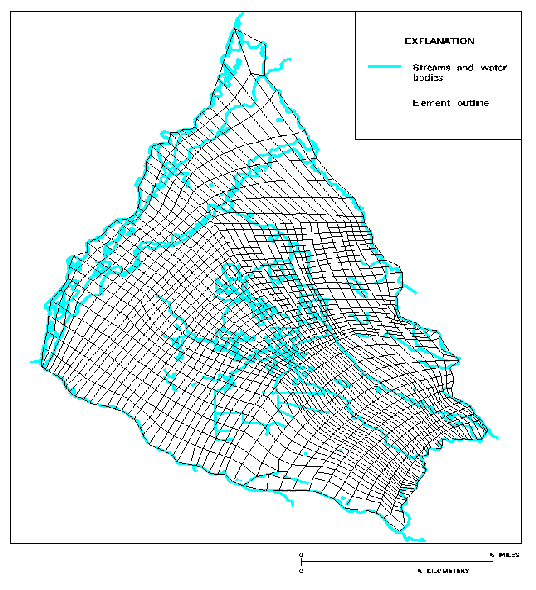
The first step to interface the finite-element ground-water flow model with ArcInfo was to convert the model mesh to a coverage. In general, ASCII files describing the mesh were loaded into INFO and manipulated through the use of INFO RELATE commands to produce ASCII files in polygon GENERATE format. The follow ing example illustrates the processing of a quadrilateral mesh (figure 1), but the same techniques were used for a mesh of triangular elements (figure 2).
The finite-element mesh was supplied as two comma-delimited ASCII files:
"id.loc"--identifiers and locations (in units of feet in the local coordinate system) for model nodes (corners of quadrilateral elements)
"el.nod"-identifiers for elements and for the corresponding nodes
Two coverages were created to represent the mesh. A point coverage of model nodes, MODELNODES, was created by applying the ARC command GENERATE to the file "id.loc." A polygon coverage of model elements, ELEMENTS, was created by applying the ARC command GENERATE to ACII files created by manipulating files "id.loc" and "el.nod" in INFO.
The files "id.loc" and "el.nod" were loaded into INFO using the INFO commands DEFINE and GET/FROM to create the data files NODE.DF and ELEMENTNODE.DF. In NODE.DF, the item NODEID is the identifier for the model nodes; the items NODEX and NODEY are the x and y locations for the model nodes. In ELEMENT NODE.DF, the item ELEMENT is the identifier for the model elements; the items NODEA, NODEB, NODEC, and NODED are the identifiers for the model nodes in a model element. The following are the first three records in the INFO data files as listed in an INFO session:
NODE.DF (1800 records)An explicit label was needed for the model elements to ensure the integrity of the identifying numbers used to link with model-calculated values. Items for x and y locations of nodes and for an estimated location of element centroids were added to the definition of ELEMENTNODE.DF. The items NODEAX and NODEAY are the x and y locations for NODEA; the items NODEBX and NODEBY are the x and y locations for NODEB; the items NODECX and NODECY are the x and y locations for NODEC; the items NODEDX and NODEDY are the x and y locations for NODED. The following is the definition of the items in ELEMENTNODE.DF as listed in an INFO session:
$RECNO NODEID NODEX NODEY 1 1 2154310.75 75603.718 2 2 2154509.00 177356.859 3 3 2155035.75 179952.046ELEMENTNODE.DF (1716 records) $RECNO ELEMENT NODEA NODEB NODEC NODED 1 1 1 2 42 41 2 2 2 3 43 42 3 3 3 4 44 43
COL ITEM NAME WDTH OPUT TYP N.DECBecause NODE.DF was sorted so that the record number ($RECNO) was the same as the node identifier (NODEID), NODE.DF could be related to ELEMENTNODE.DF by each of the node identifiers in ELEMENTNODE.DF using the RELATE command with the LINK option to bring the locations of the nodes into the ELEMENTNODE.DF:1 ELEMENT 4 4 I -
5 NODEA 4 4 I -
9 NODEAX 10 10 N 2
19 NODEAY 10 10 N 3
29 NODEB 4 4 I -
33 NODEBX 10 10 N 2
43 NODEBY 10 10 N 3
53 NODEC 4 4 I -
57 NODECX 10 10 N 2
67 NODECY 10 10 N 3
77 NODED 4 4 I -
81 NODEDX 10 10 N 2
91 NODEDY 10 10 N 3
101 CENTERX 10 10 N 2
111 CENTERY 10 10 N 3
For each element, the location of the label point was estimated to be the arithmetic mean of the node locations. This estimated location will always be within the element polygon because the model requires elements to be regular polygons.ENTER COMMAND >RELATE NODE.DF BY NODEA LINKENTER COMMAND >CALC NODEAX = $1NODEXENTER COMMAND >CALC NODEAY = $1NODEYENTER COMMAND >RELATE NODE.DF BY NODEB LINKENTER COMMAND >CALC NODEBX = $1NODEXENTER COMMAND >CALC NODEBY = $1NODEYENTER COMMAND >RELATE NODE.DF BY NODEC LINKENTER COMMAND >CALC NODECX = $1NODEXENTER COMMAND >CALC NODECY = $1NODEYENTER COMMAND >RELATE NODE.DF BY NODED LINKENTER COMMAND >CALC NODEDX = $1NODEXENTER COMMAND >CALC NODEDY = $1NODEY
ENTER COMMAND >CALC CENTERX = ( NODEAX + NODEBX + NODECX + NODEDX ) / 4
ENTER COMMAND >CALC CENTERY = ( NODEAY + NODEBY + NODECY + NODEDY ) / 4
An ASCII file that contained the element identifier (ELEMENT), the label location (CENTERX and CEN TERY), and each of the node locations (NODEAX and NODEAY, NODEBX and NODEBY, NODECX and NODECY, and NODEDX and NODEDY) was printed so that the file was in polygon GENERATE format.
ENTER COMMAND >CALC $COMMA-SWITCH = -1ENTER COMMAND >OUTPUT POLYLIST.FIL
ENTER COMMAND >PRINT ELEMENT,',',CENTERX,',',CENTERY,*L1,
NODEAX,',', NODEAY,*L1,NODEBX,',',NODEBY,*L1,NODECX',',
NODECY,*L1,NODEDX,',',NODEDY,*l1,'end'
To complete the GENERATE-formatted file "polylist.fil", the word "end" was added to end of the file "polylist.fil." A polygon coverage was created by applying the ARC command GENERATE to the file "polylist.fil" and then applying the ARC command CLEAN to create topology.
Figure 1. Model mesh of irregular quadrilateral elements.
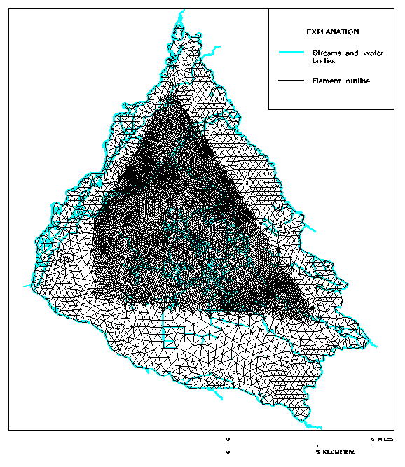
Figure 2. Model mesh of irregular triangular elements.
Because hydrologic features influence hydraulic properties, their location influences the design of the finite- element mesh. Model-node locations, as represented in MODELPOINTS were moved in ARCEDIT to more closely align with geographic features such as streams (figure 3). The corrected point locations were provided to the model as edited ARC UNGENERATE files. A new polygon coverage was created from the corrected model- node locations.
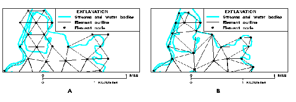
Figure 3. Model mesh (A) before and (B) after editing model-node locations to more closely align with geographic features.
Data from different sources were combined to create an integrated surface represented by a tin that then was provided as input to the model. The following example illustrates the integration of two data sources, a file and a coverage, to interpolate values at the model nodes.
"thick"--a comma-delimited ASCII file of saturated thickness at the centroids of elements, in order of element identifier but not including the element identifierTHICKCON--a line coverage of contours at 10-foot intervals of saturated thickness within a subset area at higher precision than values in "thick"
The file "thick" was loaded into INFO using the INFO commands DEFINE and GET/FROM to create THICK.DF. The outer boundary of THICKCON was digitized to create THICKBND, a polygon coverage. This digitizing was on screen, using end points of contour lines as a guide. The polygon labels for ELEMENTS were moved to the geometric centroid of each element, using the ARC command CENTROIDLABELS, and a point cov erage CENTROIDS was created from those labels, using GET in ARCEDIT. An item for saturated-thickness value was added to the polygon attribute table (PAT) for CENTROIDS using the ARC command ADDITEM.
Because THICK.DF was sorted so that its record numbers were the same as the element that the thickness represented, THICK.DF could be related to CENTROIDS.PAT by the element identifier in CENTROIDS.PAT using the INFO command RELATE with the LINK option to bring the thickness values into the coverage PAT.
ENTER COMMAND >SEL CENTROIDS.PATENTER COMMAND >RELATE THICK.DF BY ELEMENTS-ID WITH LINK
ENTER COMMAND >CALC THICKNESS = $1THICKNESS
Two tins were created using the ARC command CREATETIN. The tin CENTR_TIN was created from the points in CENTROIDS to represent a surface of values for saturated thickness outside of THICKBND. The tin CON_TIN was created from the lines in THICKCON to represent a surface of values for saturated thickness within THICKBND.
Arc: createtin CENTR_TINValues of saturated thickness were interpolated at the model nodes.Createtin: cover CENTROIDS point thickness
Createtin: cover THICKBND poly # softerase
Createtin: end
Arc: createtin CON_TIN 1 1
Createtin: cover THICKCON line contour
Createtin: cover THICKBND poly # softclip
Createtin: end
Arc: tinspot CENTR_TIN MODELNODES centr.thick quinticArc: tinspot CON_TIN MODELNODES con.thick quintic
The model-node identifiers and the interpolated values of saturated thickness were printed into two ASCII files.
ENTER COMMAND >SEL MODELNODES.PATENTER COMMAND >RESEL CENTR.THICK NE -9999
ENTER COMMAND >OUTPUT CENTR.FIL
ENTER COMMAND >PRINT MODELNODES-ID,',',CENTR.THICK
ENTER COMMAND >RESEL THICKCON.THICK NE -9999
ENTER COMMAND >OUTPUT CON.FIL
ENTER COMMAND >PRINT MODELNODES-ID,',',THICKCON.THICK
The two files, "centr.fil" and "con.fil", were combined into an INFO data file using the INFO commands DEFINE and ADD/FROM. The following are the item definitions for that INFO data file.
NODETHICK.DF (1730 records)The INFO data file was sorted by ascending model-node identifier, and an integrated ASCII file, "thickness," was printed for input into the model.COL ITEM NAME WDTH OPUT TYP N.DEC
1 NODEID 4 4 I -
5 THICKNESS 4 12 F 3
ENTER COMMAND >SORT ON NODEIDENTER COMMAND >OUTPUT NODETHICK.FIL
ENTER COMMAND >PRINT NODEID,',',THICKNESS
Model-calculated values, such as simulated hydraulic head, residuals between measured and simulated hydraulic head, discharge from the ground-water system, and recharge to the ground-water system, were displayed in ArcInfo with other coverages, such as hydrography, geology, and political boundaries, for evaluation. The values from the model were supplied as comma-delimited ASCII files. Model-calculated values were loaded into ArcInfo and converted to tins, using the same method described in the "Integration of Data" section to convert "thick" into a tin.
Although saturated thickness was not a model-calculated result, the saturated thickness example is continued for clarity. The tins created from model-calculated values were converted to line coverages of con tours, using the ARC command TINCONTOUR; then the coverages were displayed using the ARCPLOT com mand ARCTEXT. For example, CENTR_TIN would be converted to a line coverage using the ARC command TINCONTOUR and then displayed using the ARCPLOT command ARCTEXT (figure 4).
Arc: tincontour CENT_TIN THICK_CON 10 0 thickness 5...
Arcplot: arctext THICK_CON contour # line 0 blank
Using the ARC command TINLATTICE, the tins were converted to raster geographic data sets (grids). The grids then were displayed using the ARCPLOT command GRIDSHADES. For example, CENTR_TIN would be converted to a grid using the ARC command TINLATTICE and then displayed using the ARCPLOT command GRIDSHADES (figure 5).
Arc: tinlattice CENT_TIN CENT_GRD quintic...
Arcplot: gridshades CENT_GRD # cent_grd.rmp
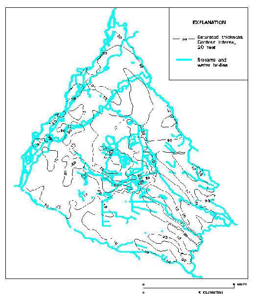
Figure 4. Saturated thickness expressed as contours.
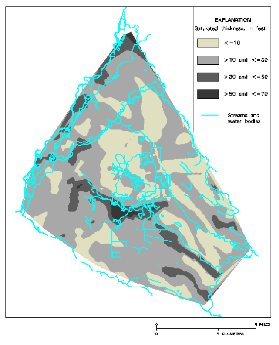
Figure 5. Saturated thickness expressed as shaded areas.
Use of a GIS can facilitate the compilation and manipulation of the large data sets often required by ground- water flow models. Data from MODFE can be transferred into ArcInfo and data from ArcInfo can be trans ferred to MODFE so that the data interpolation, integration, and display capabilities of ArcInfo can be used.
Cooley, R.L., 1992, A MODular Finite-Element model (MODFE) for areal and axisymmetric ground-water-flow problems, part 2: derivation of finite-element equations and comparisons with analytical solutions: U.S. Geological Survey Techniques of Water-Resources Investigations, Book 6, Chapter A4, 108 p.
Price, C.V., and Pierce, R.R., 1994, GIS Applications to hydrologic modeling in the U.S. Geological Survey, Water Resources Division: Past and Future, in Proceedings of the Fourteenth Annual Esri User Conference, p. 1163-167.
Torak, L.J., 1992a, A MODular Finite-Element model (MODFE) for areal and axisymmetric ground-water-flow problems, part 1: model description and user's manual: U.S. Geological Survey Open-File Report 90-194, 153 p.
Torak, L.J., 1992b, A MODular Finite-Element model (MODFE) for areal and axisymmetric ground-water-flow problems, part 3: design philosophy and programming details: U.S. Geological Survey Open-File Report 91-471, 261 p.
Jennifer B. Sieverling, Hydrologist
U.S. Geological Survey, Water Resources Division, Colorado District
Box 25046, MS 415, Denver Federal Center
Denver, Colorado 80225
Telephone: (303) 236-4882, Fax: (303) 236-4912
E-mail: jbsiever@usgs.gov
Stephen J. Char, Hydrologist
U.S. Geological Survey, Water Resources Division, Colorado District
Box 25046, MS 415, Denver Federal Center
Denver, Colorado 80225
Telephone: (303) 236-4882, Fax: (303) 236-4912
E-mail: sjchar@usgs.gov