Benjamin J. Sherman
Mark J. TenBroek, P.E.
Hydrologic and Hydraulic Computer Model Parameter Distribution, Projection, and Correlation Development Using a Geographic Information System
Abstract
Coupled hydrologic and hydraulic models have been developed for the Detroit Water and Sewerage Department's long term combined sewer overflow (CSO) control plan. Data were collected from a variety of sources in several different formats. To best manage this data, a GIS was developed to support the model. This paper addresses one aspect of the use of GIS to support models - the establishment of parameter correlations and distribution and projection methods. Previous versions of the model used coarsely defined model parameter information. The GIS that was developed provided an efficient means to enhance the resolution for three important model parameters: dry weather flow (DWF), directly connected impervious area (DCIA), and rainfall dependent inflow and infiltration (RDII).
The parameter estimates produced using the GIS were incorporated in the Greater Detroit Regional Sewer System (GDRSS) model. The model was validated using a large quantity of measured system flows and levels. In addition to increased resolution, the GIS provided a method to rapidly project this information to anticipated future conditions. This was particularly useful since the model is the primary tool for evaluating long term CSO control alternatives. Furthermore, the GIS can support other options including refinement of additional parameters, expansion of the model to consider water quality, and updating existing information as new information becomes available.
1 Introduction
1.1 Background
The City of Detroit, Michigan, developed a regional sewer collection system Stormwater Management Model (SWMM) to assist in developing the best approach to reduce combined sewer overflow discharges. A combined sewer collects both stormwater and sewage. When stormwater runoff occurs at a sufficiently high rate, the capacity of the combined sewer system will be exceeded and discharges will occur from overflow points to the receiving waters. These discharges result in a variety of problems including aesthetic problems, bacterial contamination, reduced receiving water dissolved oxygen levels, and deposition of solids. Many of these problem can impact aquatic life.
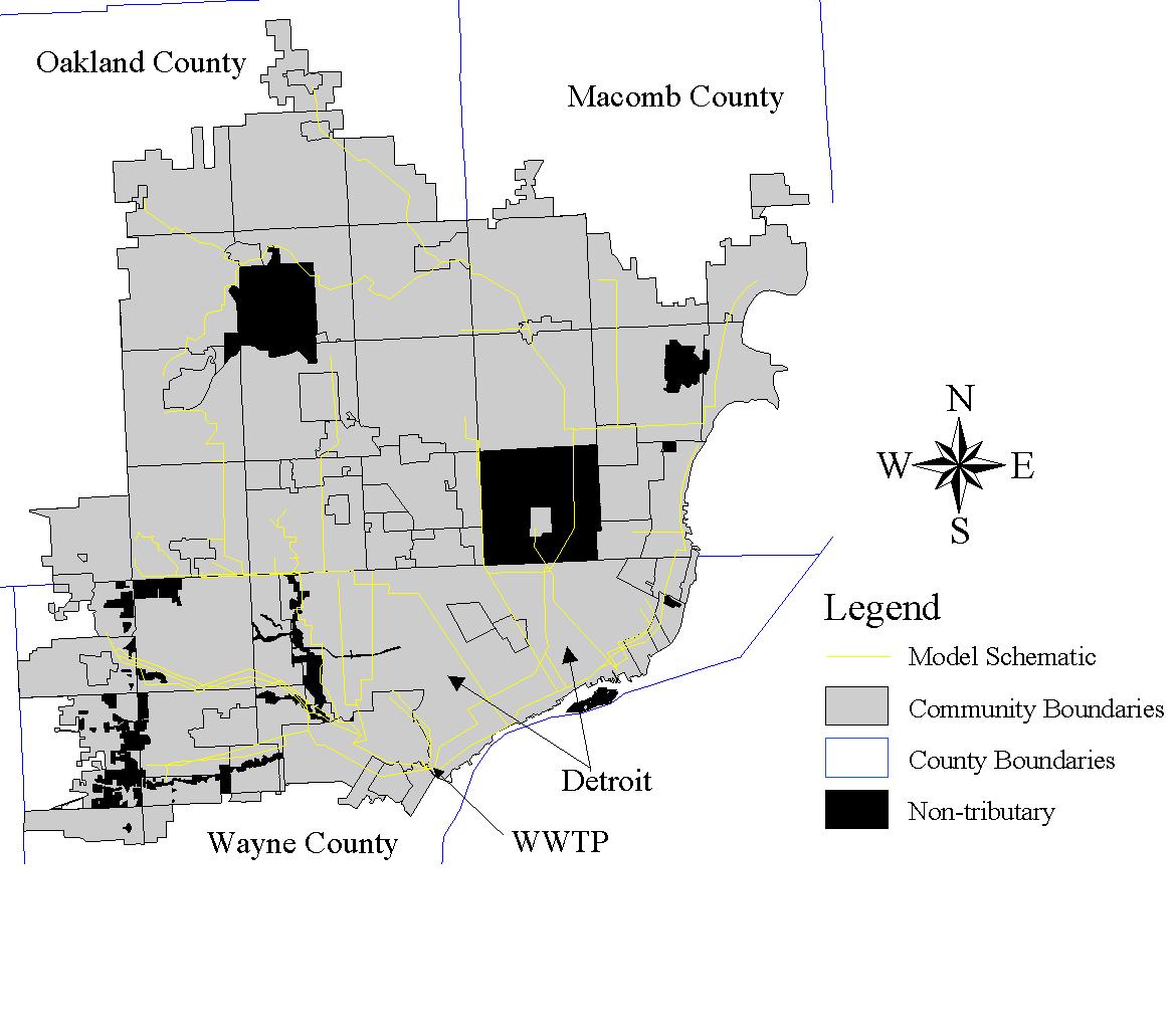
The GDRSS collection system includes the City of Detroit and all or part of 76 surrounding communities, extends over 900 square miles, and serves nearly three million people. The hydrologic model that has been prepared consists of 337 distinct subbasin drainage areas, and the hydraulic model consists of over 3,200 explicitly modeled conduits. The GDRSS model has been under development since 1988. Figure 1.1 shows the model schematic and the GDRSS tributary area community boundaries.
Figure 1.1 GDRSS Model Schematic and Boundaries for Tributary Communities
The purpose of this paper is to present the most recent improvement made using the GIS to improve the estimation, distribution, and projection of three important modeling parameters. Previous phases of model development and evaluation resulted in the conclusion that there was a need to provide greater refinement in some of the model parameters to account for the spatial and seasonal variation seen in the collected flow and level data. For a modeling project of this size, refinements such as these can only be accomplished in a cost and time efficient manner by utilizing GIS tools. During the current project, a significant amount of additional data was collected throughout the model tributary area to support these efforts. This data provided insight into spatial variation of the DWF, DCIA, and RDII.
The fundamental spatial unit used with the hydrologic model are subsections of the sewer system tributary area. These spatial units, described as polygons, were designated as the fundamental GIS data unit. Once this foundation was in place, information from existing coverages, flow and precipitation data analysis results, and system and model information were used to complete the model GIS. The GIS was also used to view tributary area statistics and determine spatial relationships for the various model parameters. Individual components of DWF were isolated to improve distribution and projection. The regional differences in DCIA were identified and variation by land use was determined using field verified data. The spatial variation of the RDII response was determined as a function of construction age for two hydrologically different time periods. Figure 1.2 shows the subbasins classified as either combined or separate sewer areas.
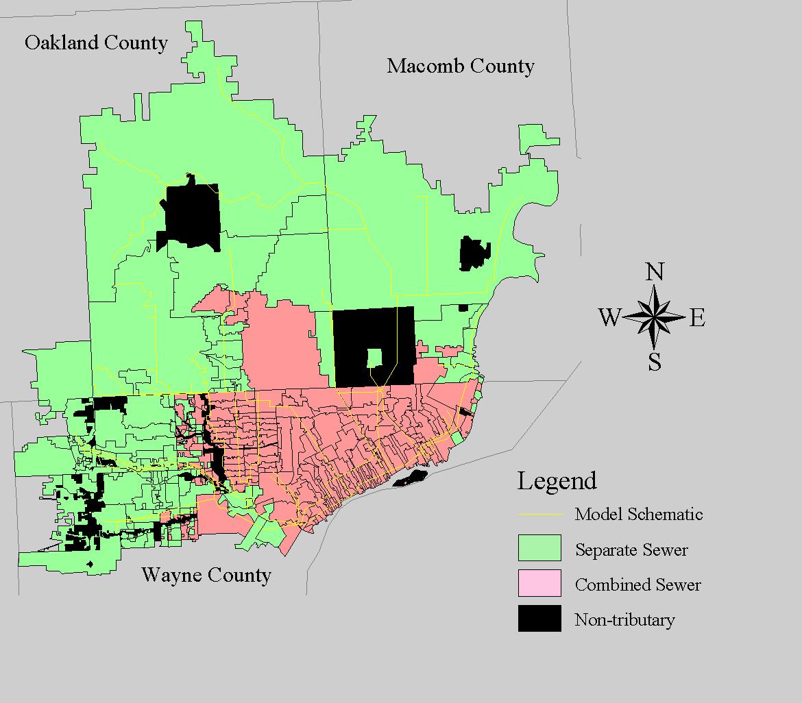
Figure 1.2 Subbasin Classification
The conclusion from this work was that the GIS parameter correlations and distribution provided greater resolution for the model input and enhanced its predictive abilities. Since the model is used to evaluate design alternatives for long term control of CSOs, the methods addressed in this paper allowed projections to future conditions based on anticipated changes in system integrity due to age, system configuration, unique features such as newly constructed CSO control basins, and expected patterns of population and employment growth and/or reduction. Furthermore, the GIS is a robust foundation for continued update and revision of the model. The GIS can easily be updated to satisfy many requirements or changes such as new census data, further parameter refinements, and additional considerations such as water quality modeling.
1.2 Definitions
Combined Sewer - Sewer systems which have the sanitary and storm sewers combined.
Combined Sewer Overflow (CSO) - Overflow stormwater and sewage from a combined sewer to a receiving water.
Directly Connected Impervious Area (DCIA) - Impervious surface areas that are directly connected to the sewer system through catch basins, roof drains, downspouts, etc. DCIA is a primary concern in combined sewer areas.
Dry Weather Flow (DWF) - Base sewer flow that does not include any wet weather derived runoff, inflow or infiltration
Evapotranspiration - The evaporation of water from land or water surface and the transpiration of water from plants
Hydraulic Model - Simulates flow routing, typically through channels and pipe networks
Hydrologic Model - Simulates the relationship of rainfall to runoff and inflow and infiltration
Rainfall Dependent Inflow and Infiltration (RDII) - Essentially all wet weather flows that enter the sewer system other than those from directly connected impervious areas. RDII is a primary concern in separate sewer areas.
Separate Sewer - Sewer systems which have the sanitary and storm sewers separate.
Subbasin - The fundamental spatial units of the computer model are subsections of the sewer system tributary area. These spatial units, polygons, are the fundamental GIS data storage unit.
SWMM - The U.S. E.P.A. Stormwater Management Model accounts for both system hydrology and hydraulics
2 GIS Development
2.1 Georeferenced Data Sources - Type
Michigan Resource Inventory System (MIRIS) - 1990 land use classification coverage
Topologically Integrated, Geographically Encoded Reference (TIGER) - 1990 U.S. Census coverage
WESSEX - base street map, political boundary, and hydrologic feature coverages
Southeast Michigan Council of Governments (SEMCOG) - 1990 employment, and 1990 to 2020 population and employment growth/reduction factors
2.2 Software
Processing: Esri ArcView and ArcCAD, and Microsoft Access
Simulation: U.S. E.P.A. SWMM GDRSS Level 2.5 and 3.0 models
2.3 Subbasin Delineation
Given the vast sewer system network it is neither financially or computationally practical to model every pipe. Therefore, after deciding which sewer pipes (primary hydraulic components) to model, the upstream characteristics of the non-hydraulically modeled system must be accurately determined and reasonably represented. The first step to characterizing the system upstream of any modeled flow inlet is to determine the planar extent of the non-hydraulically modeled system. These areas are subsections of the sewer system tributary area called subbasins. A subbasin is used to account for both the non-hydraulically modeled sewer system as well as to characterize all the hydrologic characteristics of the system.
From sewer section maps, modeled flow inlet points can be identified and upstream reaches of the sewer network defined. Any area adjacent to these upstream pipes which likely impacts the system hydrologically is considered part of the subbasin area. Hydrologic impacts are those which produce flows to the system from sources that are part of the hydrologic cycle. For example, rainfall may infiltrate the ground where sewer pipes having poor joint integrity receive this additional flow. Also, the rainfall may enter the sewer network from impervious surface runoff, such as a street that drains into a catch basin connected to a combined sewer.
3 Trends and Correlations
Once the GIS was established, ArcView plots were generated showing various spatial statistics such as population, income, housing age, combined and separate sewer areas, and land use. Also, tables were generated summarizing statistics by tributary area, billing districts, communities, and subbasins.
3.1 Dry Weather Flow (DWF)
Information regarding dry weather flows by districts were compared using these summary tables. The comparison suggested that residential population would be a logical distribution statistic. After preliminary work began using population, the need to account for flows in highly industrial/commercial sectors of the system became apparent. Therefore, employment data was chosen to account for these spatial information gaps.
3.2 Directly Connected Impervious Area (DCIA)
From previous project work, DCIA was known to vary by regions and within region by land use. The tributary area could be segmented into regions of similar characteristics based on land use, DCIA trends, and knowledge of the region's development history and unique characteristics. For example, most of the stormwater runoff from freeways within Detroit is collected by the combined sewer system; whereas, swales collect the greater portion of the runoff in the suburban areas. Also, about 70 percent of the downspouts in the oldest residential combined areas were directly connected to the collection system. Only 50 to 60 percent were connected in the newer suburban combined areas..
3.3 Rainfall Dependent Inflow and Infiltration (RDII)
From previous work (Sherman et al), sewer construction age and system network density were characteristics related to the RDII volume. The older, leakier systems naturally yielded more RDII. Likewise, more leakage is expected from the denser network of pipes due to the larger number of connections per subbasin area. The RDII parameter values were collected from a total of 70 areas that ranged from approximately 25 to 12,000 acres in size. Correlations were established to estimate the RDII in areas where data were not available. The 1990 U.S. Census GIS coverage statistic for median building age was used as a surrogate for sewer system age. This GIS coverage provided an estimate for sewer system age at the census block group level.
These correlations were used to develop the RDII C factors for two distinct seasonal periods of the year. A dormant period (Winter/Spring) in which little evapotranspiration occurs and groundwater levels are typically higher, produces more RDII than during the growth period (Summer/Fall). An RDII C factor is the slope of the RDII volume versus precipitation volume plot. The RDII C factor is one of the input parameters required to characterize RDII in the model.
Figure 3.1 shows the results of these correlation analyses. Extrapolation was not permitted from these correlations. For subbasins exceeding a 40-year construction age, RDII C factors of 15% and 8% were used for the dormant and growth periods, respectively. Where data were available, the measured RDII supersedes the correlation derived value. Equations 1 and 2 describe the best fit correlations for the dormant and growth period RDII C factors to the construction age surrogate, respectively. The coefficients of determination for Equations 1 and 2 are 0.79 and 0.70, respectively.
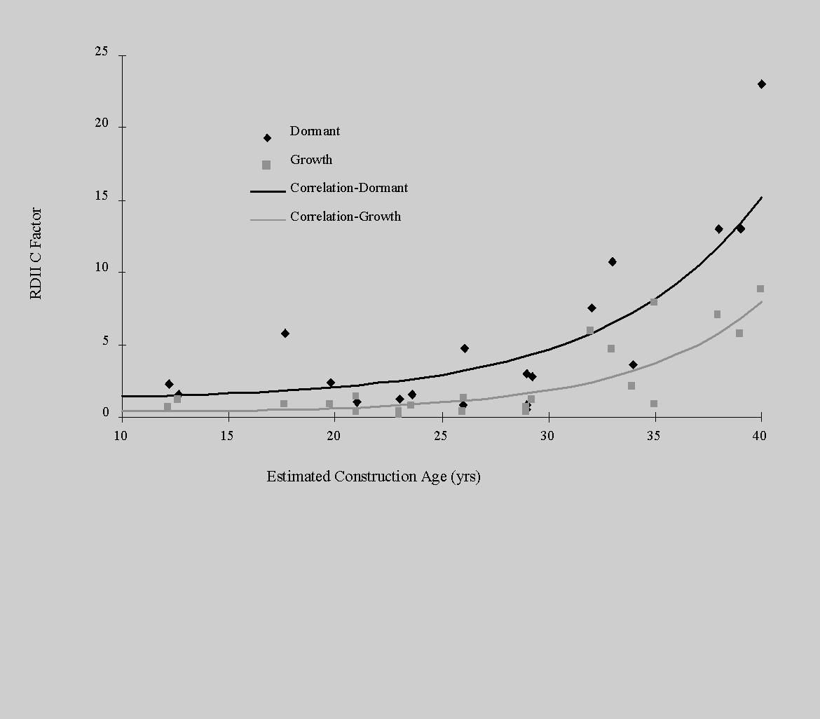
Figure 3.1 RDII Correlation to Surrogate for Construction Age
Dormant: RDII C (%) = ![]() (1)
(1)
Growth: RDII C (%) = ![]() (2)
(2)
4 Distribution Methods
4.1 Dry Weather Flow Distribution
Available sewage flow data was collected from the suburban communities and the City of Detroit wastewater treatment plant (WWTP) for the period from November, 1992 through October, 1993. Precipitation data was also collected for this same period from six gages covering the tributary area. The precipitation data was collected to assist in identifying the wet weather flow data. Flow data were classified as occurring on either a wet or dry day. A wet day was considered to be any day in which a meter's corresponding rainfall gage recorded precipitation. Furthermore, to account for longer term wet weather influences on the system such as inflow and infiltration, one or two subsequent days were classified as wet days in addition to the day on which precipitation was recorded. Once the wet weather flows were determined, the dry weather flows were determined from the balance of the flows.
After these system-wide DWFs were calculated, a flow balance was performed to determine the unmetered flow areas. The unmetered areas included the Cities of Hamtramck, Highland Park, the City of Detroit, parts of Harper Woods, Redford Township, and the City of Dearborn. A total of 18 dry weather flow districts with their respective dry weather flow data were used in this analysis. For the most part, DWF district boundaries coincided with billing districts. Flows determined for each DWF district provided a coarse distribution of the DWF. The next step was to distribute these flows within the districts at the subbasin level.
Once the total flow was calculated for each district, the flow components were identified. Flow components were required to equitably distribute the flows within each DWF district and to provide a basis on which to estimate base flows resulting from system expansion or customer base reduction. As a result, it was assumed that a change in the portion of base flow attributable to population is proportional to an increase in population. With further investigation other significant flow components were identified. The following DWF components were isolated and expressed in the flow balance equation (3):
Qtotal = Qp + Qi + Qe + Qr + Qf (3)
4.1.1 Dry Weather Flow Attributed to the Residential Population
Sewered residential population was obtained from the TIGER 1990 U.S. Census data coverage. Sewered populations were calculated as the ratio of sewered housing units to total housing units multiplied by the total population. Next, a sewered population density was added to the same coverage. The census coverage was then intersected with the subbasin coverage. The resulting coverage populations were calculated using the population densities and the new areas. The populations were summed for each subbasin and each dry weather flow district.
Through analysis of flow data from small residential study areas, it was determined that residential flows are approximately 120 gallons/capita/day (gpcd). The estimate of 120 gpcd and the populations at the subbasin level were used to determine the DWF component attributable to the residential population in each subbasin. Then the 120 gpcd estimate and the population values were used to determine the DWF component attributable to the residential population for each district. The district flow due to the residential population was required to determine the "fixed" flow component discussed later in this paper.
4.1.2 Dry Weather Flow Attributed to Specific Significant Industrial Users
The Detroit Water and Sewerage Department (DWSD) maintains a database of 351 significant industrial users. These industrial users were considered because they contribute approximately 7.7 percent of the total dry weather flow recorded at the WWTP. In some cases these industries are located in isolated areas and generate significant flows. From the database of industrial users, only industries that exceeded both 0.1 mgd and 100 gallons/employee/day were considered in this analysis. This criteria reduced the data to 54 significant industrial users contributing from 0.15 to 7.50 cfs at 112 to 19,400 gallons/employee/day. These 54 industries affected flows in 39 subbasins and accounted for 5.0 percent of the total dry weather flow in 1995.
4.1.3 Dry Weather Flow Attributed to the Employed Population
A hybrid TIGER 1990 U.S. Census data employment coverage was created to support this work. The hybrid utilized a SEMCOG employment database which classified employment zones as aggregates or subsections of U.S. Census block groups. The employment information was added to a copy of the census coverage using relational database commands and minor changes to the coverage topology. Once the employment coverage was created, the DWF component attributable to the employed population was determined using the same method as that described for the residential population flows. However, a value of 20 gallons/employee/day (gped) was used to assign flows instead of the 120 gpcd used for the residential population DWF.
The 20 gped was determined by evaluating the 351 Significant Industrial User database flows. The lowest ten percent in terms of flow per employee per day was found to be approximately 20 gped. This value was assumed representative of most industry and commerce. Using the 20 gped and the employment at the subbasin level discretization, the DWF component attributable to the employed population for each subbasin was determined. Furthermore, using the 20 gped and the employed population at the district level, the DWF component attributable to the employed population for each district was determined. The district flow due to the employed population was required to determine the "fixed" flow component discussed in a subsequent section of this paper. If a subbasin or district also contained significant industrial user flow, the significant industrial user employee count was first subtracted from the subbasin employee count to avoid double counting of flow.
4.1.4 Dry Weather Flow Attributed to River Inflow
The river inflow component was more difficult to quantify. The majority of river inflow most likely occurs sporadically throughout the system after storm events in which submerged outfall backwater gates are lodged open by debris. Another consultant working on these backwater gate systems provided an estimate of river inflow for tightly closed backwater gates as 0.26 mgd for the entire collection system. An earlier study performed in the early 1980s estimated total river inflow as 41 mgd. The river inflow chosen was 14.7 mgd and was based on both studies and an assumed limitation on inflow after storm events. The 14.7 mgd was distributed equally to 19 specific subbasin areas located along the Detroit and Rouge Rivers.
4.1.5 Dry Weather Flow Attributed to "Fixed" Flow
The "fixed" flow constitutes the balance of the flow components. The total district flow minus all other district flow components previously determined equals the "fixed" flow. This term is primarily an unidentified flow component used to balance measured flows with the component flow values. However, this flow component does provide a means to account for a portion of the base flow which does not change with system expansion or customer base reduction. Furthermore, variation in this term between DWF districts may be due to inflow and infiltration differences. The older districts of the tributary area tend to exhibit higher "fixed" flow which would correspond to older sewer materials and outdated construction methods. Once the quantity of "fixed" flow was determined for each district, it was distributed to each subbasin based on area weighting.
4.2 Directly Connected Impervious Area Distribution
To distribute DCIA, land use information, similar region delineations, and DCIA values corresponding to land use classification by region were required. The DCIA parameter was required for subbasins which represented combined sewer areas only. Regions that have similar characteristics with respect to DCIA were delineated. Ten DCIA classification regions were identified for the system. A land use coverage maintained by the State of Michigan was obtained which consisted of 66 land use classifications. These land use classifications were aggregated into the following ten for simplification:
Land Use Classification Percent of Tributary Area
Forest/Rural Open 17.1
Urban Open 3.8
Agriculture/pasture 5.3
Low Density Residential 10.5
Medium Density Residential 36.3
High Density Residential 3.0
Commercial 10.5
Industrial 7.7
Highways 1.9
Water/Wetlands 3.9
In addition, approximately 350 DCIA values estimated from flow and field sources were identified. Of these data, 117 values pertained to residential land use areas. DCIA values were assigned to each land use classification by DCIA region. The land use coverage was then intersected with the subbasin coverage to obtain land use statistics by subbasin. A single DCIA value for each combined subbasin was determined by area weighting as expressed in equation (4).
Where, Ai is the area of land use classification i, DCIAi is the DCIA assigned to a specific land use classification for a DCIA region, and AT is the total subbasin area. (4)
4.3 Rainfall Dependent Inflow and Infiltration Distribution
The distribution of RDII parameters at the subbasin level required the previously mentioned correlations and housing unit age. Again, housing unit age was used as a surrogate for sewer system age. The RDII parameters were required for subbasins which contained separate sewer areas only. A weighted average median housing unit age was obtained for each subbasin area by using the TIGER 1990 U.S. Census data coverage intersected with the subbasin coverage.
A significant number of TIGER polygons did not have data for median housing unit age. Therefore, the area weighting of median housing unit age was sometimes based on the total area of available data and not necessarily the subbasin total area. The area weighting was easily performed using the project database with the appropriate conditions and aggregate function. Once a representative housing unit age was calculated, the two correlations were used to obtain the RDII C factors for both dormant and growth seasons for each subbasin.
5 Parameter Projection Methods
Since the model is being used to evaluate long term CSO control alternatives, consideration of system conditions in future years is critical. A number of model parameters have been modified to account for these anticipated changes in system conditions. Three projection levels were generated. A 1995 level was used for the calibration and validation requirements. The calibration and validation processes utilized measured 1995 flow and level data. A 1998 level was used to evaluate a large number of CSO control projects that will be completed in that year. A 2020 level model has been generated for long term analyses.
5.1 Dry Weather Flow Projection
Anticipated population and employment growth and reductions information was obtained from the SEMCOG 2020 Regional Development Forecast: Summary Report. This report presented growth and reduction factors of population and employment by community from 1990 to 2020. The WESSEX political boundary coverages for cities and townships were used to generate a single political boundary coverage for the tributary area. The SEMCOG factors were added to the composite political boundaries coverage. The political boundaries coverage was then intersected with the subbasin coverage. Again, area weighting was applied to assign growth and reduction factors for employment and population at the subbasin discretization level.
The growth and reduction factors were then applied to each of the 18 DWF districts' residential and employed populations. The significant industrial user, river inflow and "fixed" flow components of DWF were assumed to remain constant for all projections. After subtracting the significant industrial user employees from the projected employment population, the projected flows due to residential and employed populations were calculated based on the 120 gpcd and 20 gped, respectively.
Given projected district flows, the distribution at the subbasin level was performed as previously described. Updated DWF projections were created for 1995, 1998 and 2020 conditions. A special case was considered for the 2020 condition. It was assumed that all housing units with septic systems (non-sewered) within the base year tributary area would have sewer connections by the year 2020. The population using septic systems was not projected since it was also assumed that growth of the number of housing units using septic systems would be negligible. Therefore, the septic system population obtained from the 1990 TIGER coverage was added to the projected 2020 population before the residential population flow was calculated.
5.2 Directly Connected Impervious Area Projection Considerations
The DCIA parameters were not adjusted for future years. DCIA is a parameter associated with older areas in the system having combined sewers. Combined sewers are no longer being constructed and, therefore, DCIA is not an issue for new growth. There is, however, one change which affects the use of DCIA in the projected models. One CSO control alternative is to separate existing combined sewer systems. Therefore, any subbasin expected to undergo sewer separation did not retain a DCIA parameter and instead was represented with RDII parameters. There were 19 subbasins that underwent sewer separation between the 1995 and 1998 projection levels.
5.3 Rainfall Dependent Inflow and Infiltration Projection
As previously mentioned, any combined sewer area that undergoes sewer separation must then have RDII parameters to characterize the subbasin. The sewer separation is primarily a rerouting of the stormwater collection system with little change to the sanitary sewer collection system. Therefore, the RDII C factor correlations to system age are assumed to be valid for a converted area. To obtain the correct system age for the projection year, correlations are used by accounting for the projected year relative to the 1990 census coverage data.
6 Results
The model GIS was developed to manage large quantities of actual system and modeled system information. One of the objectives of using the GIS was to distribute and project three important model parameters. The distribution and projection methodologies have been discussed. As with many GIS applications, the results are best presented graphically. Figure 6.1 shows the dry weather flow district boundaries. Figure 6.2 shows DWF densities for the GDRSS tributary area by subbasin for the 1998 projection year. Flow density is expressed as cfs/acre to view the relative spatial differences. For comparison, Figure 6.3 shows the DWF densities for the GDRSS tributary area by subbasin for the 2020 projection year. Between 1998 and 2020, one notices the majority of growth occurred in the suburban communities.
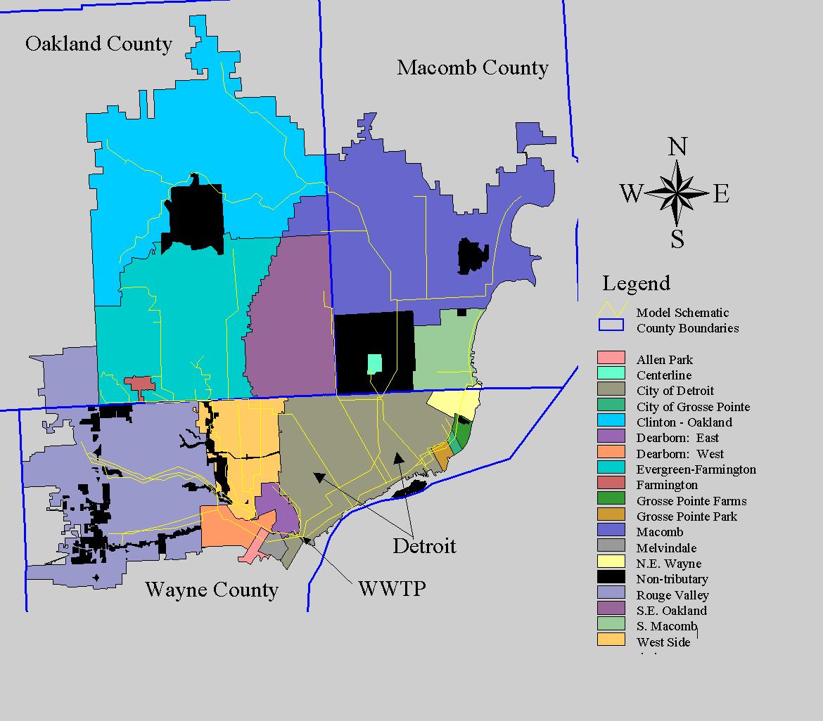
Figure 6.1 Dry Weather Flow Districts
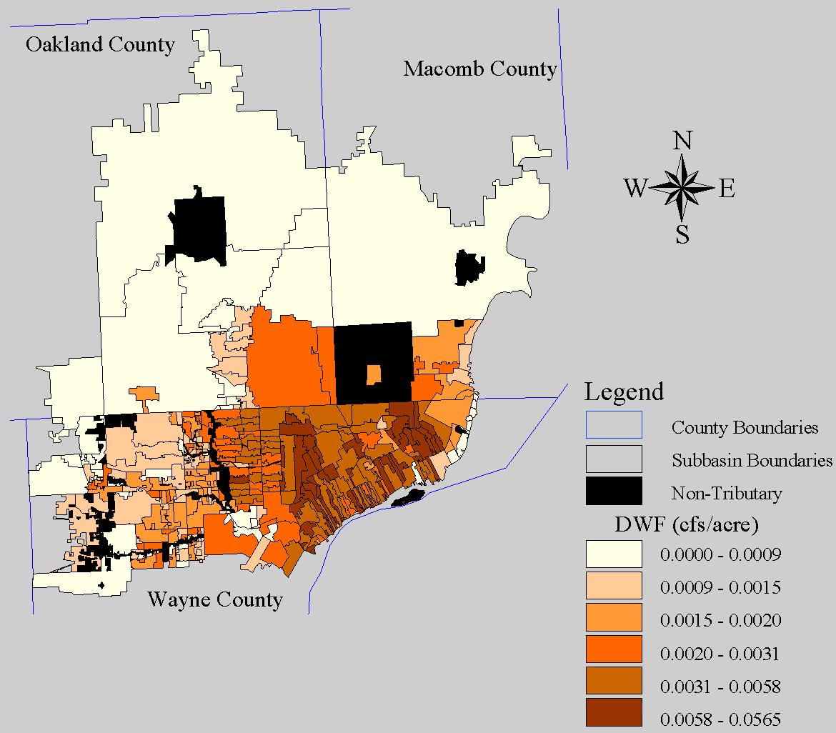
Figure 6.2 1998 Dry Weather Flow Density
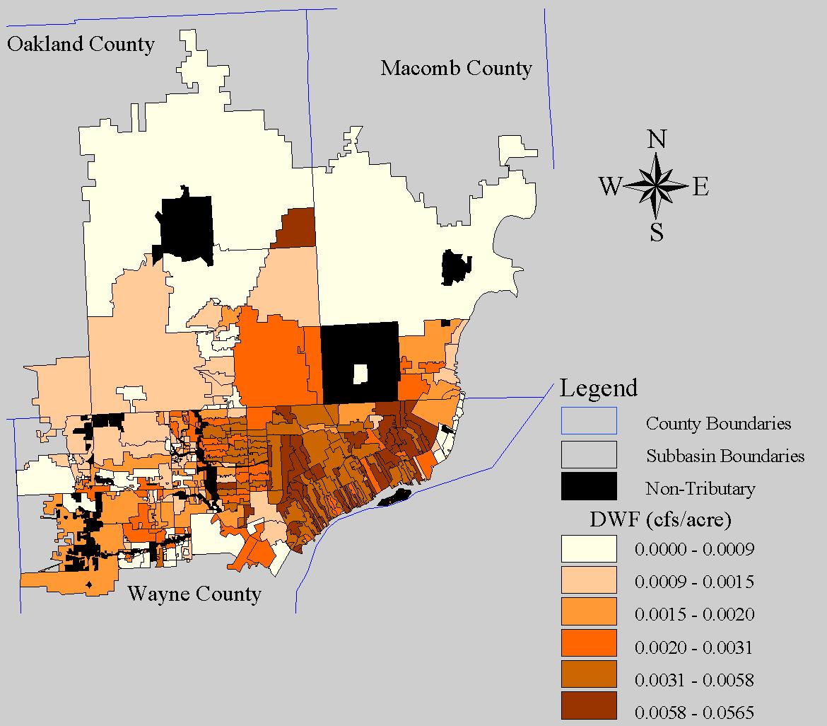
Figure 6.3 2020 Dry Weather Flow Density
The DCIA by subbasin are shown in Figure 6.4. The graphic shows large values for DCIA in the downtown Detroit area, as is typical of highly urbanized regions. Each combined sewer subbasin has a discrete DCIA which is used as input to the model. One notices that there are few combined sewer subbasins to the west of the City of Detroit, yet there a number of DCIA regions defined. As previously mentioned, the 1998 level model represents 19 sewer separation projects, of which most were in Western Wayne County.
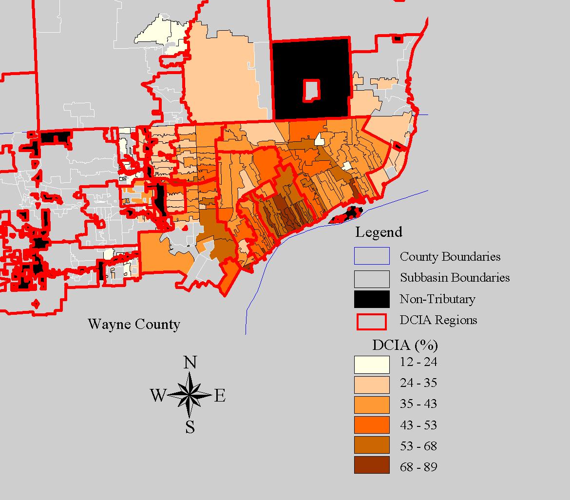
Figure 6.4 1998 DCIA by Subbasin (Combined Sewer Only)
The RDII C factors by subbasin for the growth season are shown in Figure 6. The graphic shows the distribution of the growth period RDII C factors throughout the separate sewer drainage areas of the model. Generally the further away from the City of Detroit, the newer the suburb construction. Therefore, the higher RDII C factors are shown in older portions of the tributary area that are closer to the City of Detroit. This is, of course, a direct function of the correlation discussed previously. A similar graphic, not shown, could be presented showing the dormant period RDII C factors by subbasin.
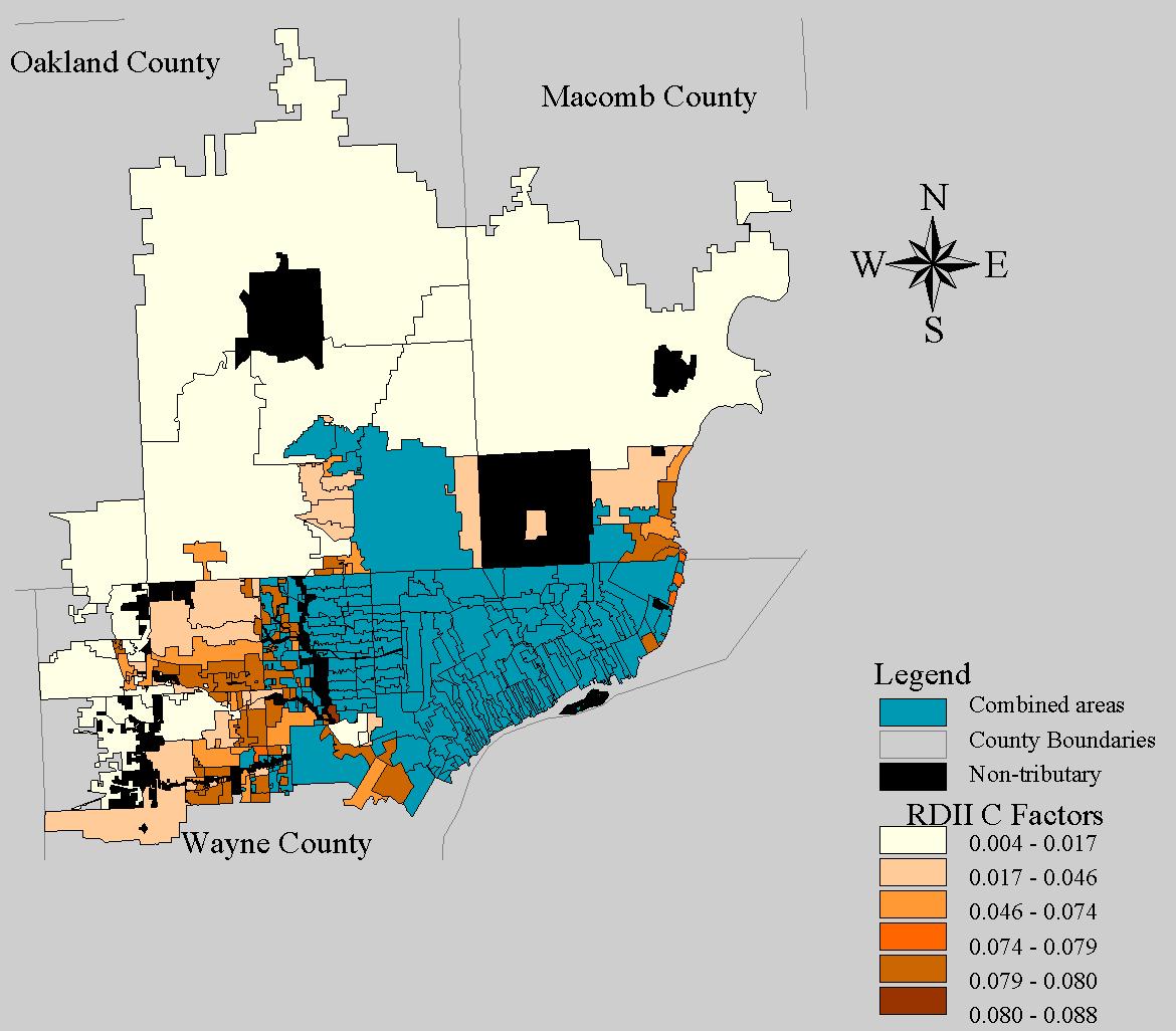
Figure 6.5 1998 Growth Period RDII C Factors by Subbasin (Separate Sewer Only)
Applying the parameters generated by the GIS to the model was relatively simple. This straightforward data extraction allowed greater flexibility in the model. That is, various complex system conditions could be represented with minimal additional work. For example, some subbasins were divided into smaller areas for greater resolution and the GIS processing work rapidly provided updated land use, population and construction age information. Through use of general database commands, the parameter data were extracted to spreadsheets for subsequent calculations using various lookup tables.
The GIS derived parameters were first incorporated in GDRSS model released in early 1996 for use on other projects. Since that time, a number of updates were made to improve the model's predictive capability. The current GDRSS model was released in early 1997. A sufficient number of changes were made with this model representation which required some redelineation of the subbasin topology, reclassification of subbasin attributes such as combined vs. separate, and repositioning of model inlet locations. The GIS was used to address these changes.
The calibration and validation of the model began during the final stages of the current GDRSS model development. The validation of the model using large amounts of measured flow and level data improved confidence in the model's predictive capability and supported the efforts made to increase model detail.
7 Conclusions
An objective of the GDRSS modeling project was to develop a GIS to support model related data management and analysis needs. An outgrowth of the GIS was to use the spatial data structure to evaluate certain critical model parameters for spatial distribution.
To satisfy the objectives leading to the parameter distribution and projection methodologies, the subbasin was identified as the fundamental spatial unit and subsequently digitized and converted to GIS. Summary data was investigated graphically and tabularly by tributary area, billing districts, communities and subbasins. Trends were identified between general statistics such as population, employment, housing unit age, land use, and the corresponding measured parameter data for DWF, DCIA and RDII. These relationships were used to develop distribution methodologies. Likewise, the data suggested a means to project much of the parameter information temporally.
The representation of DWF, DCIA and RDII in the GDRSS model has been improved. The previous versions of the model incorporated a coarse distribution using a lesser quantity of data. The GIS provided for greater data management capability and a means to significantly enhance the model refinement. The projection methodology allows for system expansion, customer base reduction, and customer base redistribution over time. Now that the model GIS tool is available, the potential for other model parameter refinement methods is improved. Updated data sets, such as the 2000 census, can readily be incorporated to adjust the parameters to more accurate information. This point should not be underestimated in value. One of the most difficult tasks in maintaining a model of this size is the ability to readily update the model with new information.
Acknowledgments
The GDRSS model development is being conducted by the DWSD. The authors of this paper would like to acknowledge Gary Fujita, P.E., Assistant Director of Wastewater Operations, DWSD, for his guidance and assistance during the several years of the development and use of this model. We are grateful for the dedication and assistance provided by Heather L. Shymanski, P.E., and Rashila Karsan, both of Applied Science, Inc., for collecting, compiling, and analyzing much of the data collected for this project. Furthermore, Satya P. Singh, Ph.D., P.Eng., of Tucker, Young, Jackson, Tull, Inc., provided valuable assistance in compiling the available data from the various projects throughout the model area.
References
Sherman, B.J., P.N. Brink, and M.J. TenBroek. Spatial and Seasonal Characterization of RDII for the Greater Detroit Regional Sewer System Model. In Proceedings, Conference of Stormwater and Water Quality Management Modeling. Computational Hydraulics International, Toronto, Ontario, February 20-21, 1997.
Author Information
Benjamin J. Sherman
Project Engineer Camp Dresser & McKee
One Woodward Avenue, Suite 1500
Detroit, MI 48226
Telephone: 313.963.1313
Fax: 313.963.3130
E-mail: SHERMANBJ@cdm.com
Mark J. TenBroek, P.E.
Associate
Camp Dresser & McKee
One Woodward Avenue, Suite 1500
Detroit, MI 48226
Telephone: 313.963.1313
Fax: 313.963.3130
E-mail: TENBROEKMJ@cdm.com
Camp Dresser & McKee
Web: www.cdm.com