Using Geographic Information Systems to Map the Strategic Value of Chesapeake Bay
Farmland: Methodology Concept of Operations
April, 1997
Abstract
The disappearance and conversion of farmland to built-up landcover types in the Chesapeake Bay area has proceeded at an aggressive rate over the past several decades. Forecasts for farmland loss are no less optimistic. Current county land use plans for the metropolitan Washington DC area forecast a loss of 309,000 acres of open lands from 1990 to 2020.
Public and private efforts to manage farmland conversion will benefit from GIS databases and maps depicting the location and extent of farmlands with high potential for controlling conversion and preserving farm landscapes. The Chesapeake Bay Foundation and the American Farmland Trust, representing the Chesapeake Farms for the Future Board, contracted with Earth Satellite Corporation(EarthSat) to develop GIS databases and a hardcopy map series as strategic tools for farmland protection and farmland conversion management for the Chesapeake Bay watershed. The purpose of this paper is to describe the technical and modeling aspects of strategic farmland mapping for the Chesapeake Bay.
EarthSat has used ArcInfo to develop multicriteria GIS databases and maps depicting the significance of Chesapeake Bay farmlands. County and statewide hardcopy maps and GIS databases representing the pattern of Maryland farmland protection, development pressure on farmland, farmland significance from a soils and nonsoils productivity perspective, farmland nonagricultural significance, and farmland water quality impact indicators have been produced. Descriptive statistics for each geographic theme were also synthesized. The map themes and spatial databases will serve as decision support tools for farmland protection management.
Data from low cost multiple sources and scales were compiled and rasterized as inputs for multicriteria modeling of farmland significance. ArcInfo GRID was applied to model farmland protection, development pressure, farmland soil and nonsoil productivity, farmland cultural, environmental and historic significance, and farmland water quality impact indicators. These models will serve as inputs to a strategic farmland model which represents farmlands of high potential value as protected farmland in controlling the conversion of farmland to developed landcover.
Data compilation management was conducted through UNIX ArcInfo, while map conversion was conducted through ARCEDIT. Raster model processing and statistical analysis was conducted through GRID. ARCPLOT was employed to generate statewide and county-level hardcopy map series. Additional statistical analysis was conducted with Microsoft Excel.
2.0 Definition of Study Areas and Enumeration Units
2.1 Proposed Map Themes
3.1 Spatial Data Sources
3.2 Additional Potential Sources of Spatial Data
4.0 Data Manipulation and Preprocessing
4.1 County-Level Map Database Preprocessing
4.2 State-Level Map Database Preprocessing
5.1 Analysis Procedures for Landuse, Zoning, and Farmland Protection Map
5.2 Analysis Procedures for Projected Development Pressure on Farmland Map
5.3 Analysis Procedures for FarmlandAgricultural Significance
5.4 Analysis Procedures for Farmland with Significant Non-Agricultural Features (Environmental, Cultural, Historic)
5.5 Analysis Procedures for Projected Subwatershed Surface Imperviousness Increase Map
6.1 Acreage Summary Tables Samples
6.2 Acreage Summary Graphs
Farmland conversion to developed and urbanized landcover within the Chesapeake Bay is of great concern. In the 1980s, the metropolitan Washington, DC region lost 211,062 acres of farmland, barren land, forests, and wetlands. This represented a seven percent decrease in the region's available open spaces. This loss is equivalent to approximately five times the area of the District of Columbia.
Forecasts show little sign that pressure to convert farmland and other open spaces to built-up landcover is receding. Between 1990 and 2020, the metropolitan Washington region is forecasted to lose 10,300 acres of open space a year. This is an additional loss of eight percent of all open space that existed in 1990. Current county land use plans for the Washington area forecast a loss of 309,000 acres of open lands from 1990 to 2020.
Forecasted loss of open space including farmlands is especially intense in the rural counties of the Metropolitan Washington area. In Maryland, between 1990 and 2020, Howard, Frederick, Calvert, and Charles counties, historically rural farming counties, are forecast to lose 144,670 acres of open space. This loss is equivalent to approximately 13 acres of open space per day. Within the metropolitan area, the historically rural farming counties of Virginia also anticipate open space loss. Loudoun, Prince William, and Faquier counties are forecast to lose 86,583 acres of open space from 1990 to 2020.
By 2020, thirty-six percent of all metropolitan Washington lands will be built-up, up from twenty eight percent of all lands in 1990. Forecast conversion of open spaces including farmlands averages to twenty eight acres per day. (1)
Planners and policymakers are confronted with a myriad of questions when planning for farmland protection against conversion. A tool for identifying location, extent, and intensity of the economic, cultural and environmental character of farm landscapes is critical to farmland protection planning.
The Farms for the Future Board, through The Chesapeake Bay Foundation and the American Farmland Trust contacted with Earth Satellite Corporation to develop a concept of operations Document for mapping the environmental and economic significance of farmland within the Chesapeake Bay.
The concept of operations was developed in coordination with the Farms for the Future Board
and Earth Satellite Corporation with a number of goals and objectives. One goal of the document
is elaborate on the feasibility of applying Geographic Information Systems (GIS) technology as a
tool for farmland protection planning. Additional goals include identifying spatial data sources
and limitations, and the costs of the application of those data for farmland significance mapping.
The concept of operation also proposes example thematic maps showing farmland significance
using currently available data and discusses the advantages and disadvantages of their
development methodology.
2.0 Definition of Study Areas and Enumeration Units
The Farms for the Future Board determined to investigate farmland significance in the Chesapeake Bay Watershed. For the purposes of the concept of operations document, the study area was limited to all of the State of Maryland. Representative sample maps for farmland significance themes were generated at the county and state levels. The Maryland Statewide map series was produced at a scale of 1:250,000 (1 cm on the map = 2.5 km ground distance, or 1 inch = ~ 3.94 miles). This scale permits production of Maryland Statewide maps not exceeding 40 inches in height.
Frederick County, Maryland was chosen as a representative county-level map for a number of reasons. In general, spatial data availability was good for Frederick County. While Frederick County has the largest physical land area in the state of Maryland, Frederick also possesses a diverse landcover landscape. Frederick County exhibits strong population growth and farmland productivity, making it a suitable study area especially for investigating the relationship of development pressure on farmland productivity. Frederick County maps are produced at a scale of 1:65,000 (1 cm = 650 meters, or 1 inch = ~1.02 miles). This scale is appropriate for generating county-level maps in a format not exceeding 40 inches in any one dimension (vertical or horizontal).
All maps produced are projected in to the Maryland State Plane Coordinate System, based on the North American Datum of 1983 and the GRS 1980 Spheroid. Metric-system measurements and distance calculations are facilitated using this meter-based system. The projection system was chosen to minimize positional error for county-and statewide maps for Maryland. Delaware county and State-level maps will also be presented in the Maryland State Plane Coordinate System, in anticipation of minimal positional error under the system.
Representative sample descriptive acreage statistics for the relevant themes were generated for
the Chesapeake Bay Watershed portions of Maryland for the State of Maryland, for Maryland
Regions, and at the County level.
Return to Table of Contents
2.1 Proposed Map Themes
A number of map themes are required to appropriately address critical decision making questions for farmland protection planning. A central goal of the project is to generate maps which identify the longevity or viability of farmland. The maps should all contribute to clarifying a concept for mapping out the strategic value of farmland within the Chesapeake Bay Watershed as a tool for protection planning.
The map themes produced should all identify the basic spatial distribution and nature of existing
farmland protection (at both the state and county level), land use, land use zoning, and public
ownership within the Chesapeake Bay. Consequently, all of these themes are represented on each
of the maps produced for this concept of operations.
Development pressure on farmland was chosen as a map theme for the purpose of identifying the distribution and pattern of population-driven development on farmlands. The intensity and spatial pattern of development pressure is an effective indicator of the threat of farmland conversion to built-up cover types and is employed as a decision making tool central to farmland protection planning.
Protection planners also need a means of assessing the value of farmlands in order to implement protections of productive farmlands. This concept of operations proposes an evaluation of farmland value in terms of both agriculture-based significance and non-agriculture based significance.
The distribution and pattern of farmland significance based on agricultural features have been identified through two map themes in this project. The first map theme, "farmland with significant agricultural features, based on soil productivity" identifies farmland significance in terms of its soil-based productivity. Soil agricultural yield and its relationship with soil suitability for agricultural use is the central map feature for this theme. The second map theme, "farmland with significant agricultural features, based on non-soil productivity" identifies farmland significance in terms of non-soil based factors. The theme focuses on farmland value in terms of the value of agricultural products sold.
Farmland significance based on non-agricultural features is also represented. A map that assesses the environmental, cultural and historic significance of farmlands is presented as a tool for evaluating farmland significance from a social perspective.
The impact of development pressure on water quality on barmland was also selected as a central issue for farmland planning protection. Projections for land surface imperviousness increase were modeled and mapped as an indicator of potential threats to farmland water quality.
The map themes presented for this concept of operations are :
The methodology employed for each of the map themes is discussed in Section 5.0, Data
Analysis.
Return to Table of Contents
3.0 Data Collection
The sources for spatial data used, the potential sources for data not used because of current
unavailability, and the fitness for use of spatial data for this concept of operations document are
discussed in this section.
Return to Table of Contents
3.1 Spatial Data Sources
A myriad of public and private organizations have been identified as sources for spatially
referenced data for this concept of operations document. EarthSat placed an emphasis on
identifying lower-cost or no-cost sources of data, especially in the public domain as a cost
controlling mechanism. As a general guideline, sources for data already in digital format for
ready import to GIS were sought out. Additional sources for non-electronic geographic
information were also identified.
The major sources of geographic information for the concept of operations hailed from the
Maryland State Government and United States Federal Government.
The Maryland Office of Planning (MOP) was a key source of electronic geographic information.
The Organization provided no-cost information for landuse, zoning, sewer service areas, soil
agricultural suitability, zoning density requirements, statistical enumeration units, population
increase forecast information, and coordinated the collection of hardcopy maps for county-level
farmland protection. This information was provided Maryland Statewide for the project.
The Maryland Department of Natural Resources (DNR) also served as a primary source of
no-cost electronic geographic information. DNR provided the project with Maryland statewide
GIS databases for state agriculture easements, preservation districts, Maryland Environmental
Trust Easements (METs), private protected lands, federally owned lands, county parks and
DNR-owned lands. Moreover, DNR provided the project with the Maryland statewide National
Wetlands Inventory (NWI) wetlands database, along with statewide flood plain data.
The federal sources of geographic information used include the United States Bureau of the
Census, the United States Geological Survey, the United States Department of Agriculture, and
the United States Environmental Protection Agency.
The US Bureau of the Census provided the project with low-cost (<$200) electronic format
attribute information for the entire US National Census of agriculture 1992 (the most current
Maryland statewide census of agriculture available). This information included complete census
data tables at the national, regional, state, county, and other census level enumeration units.
Census farm count information at the ZIP code level for the entire US was also provided.
The US Census TIGER/LINE geographic information database served as a significant low-cost
source for basemap information. Spatial data for state, county, and ZIP code boundaries,
placenames and landmarks, interstates, highways, streets and roads, and rivers and streams were
extracted from US Census TIGER/LINE.
The United States Geological Survey (USGS) also served as a no-cost source for a wide
assortment of electronic spatial data. US national hydrological units for defining the Chesapeake
Bay Watershed, along with digital elevation models and ancillary wetland landcover were
obtained from the USGS at no cost over the internet.
The National Soil Survey Center of the Soil Conservation Service in the United States
Department of Agriculture was an additional no-cost source of electronic spatial data. The
organization's State Soil Geographic (STATSGO) Data Base was a no-cost consistent source of
electronic format soil yield information for the entire US.
The United States Environmental Protection Agency provided the project with a no-cost
Chesapeake Bay shoreline map database.
The University of Maryland at Baltimore County and the Baltimore-Washington Regional
Collaboratory provided no-cost multi temporal landcover data used in modeling development
pressure and locating zones of conflict that identify areas of potential farmland conversion.
The Delaware Department of Agriculture, along with Thompson Mapping provided low-cost
CAD format spatial data for Delaware agriculture land suitability, environmental features, and
wastewater service areas. The planning offices for Kent, Newcastle, and Sussex Counties,
Delaware each provided spatial data or sources for spatial data for county-level zoning
information. The Delaware Department of Economic Development also provided zoning spatial
data. The Delaware Department of Health and Social Sciences provided consistent Delaware
statewide population and household increase forecasts. Maps for Delaware were not produced for
this concept of operations document.
Statewide placenames information was derived from Environmental Systems Research Institute's
(Esri) 1:2,000,000 ARC/USA spatial database.
County-level farmland protection in the form of Transfer of Development Rights (TDRs) and
Purchase of Development Rights (PDRs) areas for Maryland was converted from county paper
maps by EarthSat technicians. The Maryland Office of Planning coordinated with EarthSat in
collection of the county protection maps.
Return to Table of Contents
3.2 Additional Potential Sources of Spatial Data
A number of additional sources were contacted through the course of the project to assess
electronic format data availability. Some sources which were in the process of producing or
updating geographic information could not distribute spatial data for this concept of operations
document until processing was completed. A number of databases with significant relevance and
useful application to the concept of operations were undergoing conversion from analog format
or were being updated or revised.
The Emergency Operations & Technical Support Program of the Maryland Department of the
Environment is in the process of converting analog farm operations information to digital format
to produce a Maryland Statewide map database of agricultural operations, food processing plants,
and wholesale/food distribution. This information would serve to enhance the Landuse, Zoning,
and Farmland Protection maps.
The Wildlife and Heritage Department of the Maryland Department of Natural Resources is
also in the process of updating their Sensitive Species Project Review Areas (SSPRA) map
database for inclusion in a forthcoming Maryland data toolbox. The Maryland Historic Trust's
Maryland Inventory of Historic Properties, National Register of Historic Places, and National
Historic Landmarks databases are not completely converted to electronic format. Maryland
scenic viewsheds, valuable in assessing the cultural value of farmland, are currently being revised
by the US Federal Scenic Highway Program, the Maryland State Highways Administration, and
the Maryland State Scenic Byways Committee. Each of these databases would serve to expand
the depth and scope of the Farmland with Significant Non-Agricultural Features maps.
The Projected Subwatershed Surface Imperviousness Increase maps would benefit from the Maryland DNR revised statewide watershed water quality database. The database is currently undergoing revision.
Return to Table of Contents
4.0 Data Manipulation and Preprocessing
All spatial databases used in the project were projected to a common coordinate system using
Environmental Research Systems Inc.'s (Esri) ArcInfo Geographic Information System
software. ARC INFO was the primary preprocessing, data analysis and cartographic software for
the project. All spatial data employed were converted to ArcInfo format (raster or vector, as
appropriate). The coordinate system used for the project is described in the following table :
Table 1. Projection Parameters Used
| Projection Parameter | Description |
| Projection: Stateplane | The projection system. |
| FIPSZONE : 1900 | Federal Information Processing Standard State Plane Zone Number. 1900 is Maryland Stateplane |
| Units : Meters | The basic unit of distance measurement in
which coordinate
information is stored. All map databases were stored in meters. |
| Datum : NAD83 | The base reference system and control points for the projection system. The North American Datum of 1983 was used. |
| Spheroid : GRS80 | The model employed approximating the shape of the earth's surface. The GRS 1980 spheroid was used |
Return to Table of Contents
4.1 County-Level Map Database Preprocessing
Beyond projection, basic preprocessing steps for data preparation for the county-level series of
maps included checking for completeness and schema consistency and conversion of vector
databases to raster structures. Consistency of attributes of each database were checked through
visual inspection of values on a map display and through generation of frequency table listings of
all possible attribute values within a vector coverage. Any apparent attribute errors were
corrected. Standardized attribute codes were added to vector attribute tables to maintain
consistency for each database.
Vector data to be used for modeling were converted to GRIDs (raster images) organized into
cells 100 meters on a side, or 10,000 square meters (1 hectare, 2.47 acres, or 107,639 square
feet) in area. The conversion used the standardized codes created in each the vector database for
grid cell value assignment. Databases converted from vector to raster structures are identified
under Section 5.0 Data Analysis. The result was a set of GRIDS for the Frederick County study
area each with 556 rows and 493 columns for a total of 274,108 cells. Conversion of the vector
database to 10,000 meter square cells produced a database spatial resolution of sufficient
generalization for 1:65,000 scale mapping. At a scale of 1:65,000, one cell, 100 m on a side is
approximately 1.53 mm in length on the map. Consequently, the spatial data produced for the
county map series should be used only at map scales of 1:65,000 or smaller.
Return to Table of Contents
4.2 State-Level Map Database Preprocessing
Preprocessing steps for data preparation for the statewide series of maps consisted of map
projection, as mentioned earlier, followed by completeness and schema consistency checks and
subsequent conversion to GRID structures. Attributes for all of the county vector databases were
checked and corrected using the same method discussed above for county data.
Following the consistency checks and correction, each county database used in the analysis was
rasterized to a cell size of 250 meters on a side, or 62,500 square meters (6.25 hectares, 15.44
acres, or 672,744 square feet) in area. The Maryland statewide study area is a lattice of 824 rows
by 1,560 columns totaling 1,285,440 cells. The rasterization step was important for the purpose
of merging the multiple databases to a common spatial resolution and for generalizing the spatial
information to a scale suitable for statewide mapping. A single 250 m cell on the Maryland
Statewide map series at 1:250,000 scale is represented as 1 mm in length. Data produced for the
Maryland statewide series should be used at map scales of 1:250,000 or larger only. Section 5.0,
Data Analysis lists the individual vector databases converted to raster format.
Since most of the Maryland data collected were organized at the county level, the statewide
series also included the additional step of interpolating landuse information where gaps between
county databases existed. When all county landuse vector databases were rasterized and merged
to form a full Maryland statewide landuse scene, small gaps of missing data between some
counties resulted. ArcInfo GRID was used to apply a majority filtering function to interpolate
for missing data. The filter converted gaps in the raster landcover data to the landcover class
found to be in the majority in the "neighborhood" or area immediately surrounding the missing
data gap. Fewer than 100 cells (or 1,544 acres in area) total were interpolated for the full
Maryland scene.
Return to Table of Contents
5.0 Data Analysis
The process of developing the methods may be considered one of evolution in the sense that at
the project outset, complex models were applied for many themes which evolved into cleaner,
simple models most suitable to meet the project goals.
EarthSat first coordinated with the Farms for the Future Board to produce a mapping method for
the county level map series. In general terms, once the concepts for the county-scale maps were
well understood, and a complete county series was generated, the county-level methods were
applied to produce statewide-level map series. For the statewide series, county-level information
was first pre-processed for the purpose of map joining, as discussed above, and then merged into
full statewide databases. Modeling techniques were then applied to the full statewide databases.
This section discusses the methodologies for generating spatial data and hardcopy maps for each
map theme.
Return to Table of Contents
5.1 Analysis Procedures for Landuse, Zoning, and Farmland Protection Map 5.1.1 Frederick County
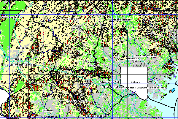
The county level Landuse, Zoning and Farmland Protection Map is designed to provide a basic spatial context for landcover, zoning, ownership, and farmland protection for county-level assessment. While the information found on the protection maps could be considered "basemap" or "background" information, they provide a fundamental context for defining the spatial character of farmland protection. The features found on the protection map will typically be found on all other map themes. The design approach to the map is cartographic overlay of multiple information layers.
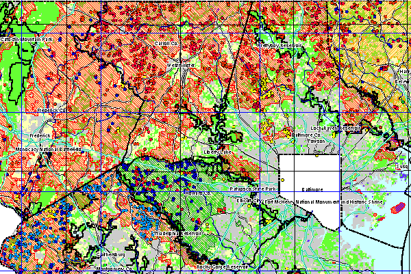
Landuse is represented as the bottommost layer (see Image 1, Detail, Frederick County Landuse,
Zoning, and Farmland Protection). Generalized landuse information for each county for 1995
was provided by the Maryland Office of Planning. Landuse types represented are
built-up/developed, agricultural landuse, forested landuse, other landuse, water, and wetlands.
State and county farmland protection are depicted on the Landuse, Zoning, and Farmland Protection Map. State protections portrayed are Maryland State Agriculture Easements, Maryland State Agriculture Preservation Districts, and Maryland State Environmental Trust Easements (METs). County farmland protection in the form of Transfer of Development Rights (Sending) areas (TDRs) and Purchase of Development Rights areas (PDRs) are also portrayed. In addition, the map shows privately held conservation areas.
To simplify information, and to avoid concealing existing landuse with opaque polygons, the
farmland protection features are symbolized with open black border polygons. Agriculture
Easements are symbolized as an open black boundary polygon with a text label "Ag E."
Maryland Agriculture Preservation Districts and Maryland State Environmental Trust Easements
are portrayed with "Ag D" and "MET" labels respectively. Likewise, TDRs and PDRs are
represented on the county Farmland Protection Map as an open polygon with a text labels "TDR"
or "PDR" respectively. Privately-owned conservation areas are labeled "Prv." State protection
and private conservation areas were provided by the Maryland Department of Natural Resources.
County protection was provided by county governments, coordinated through the Maryland
Office of Planning, and converted by EarthSat digitizing services. (2)
Image 1, Detail, Frederick County Landuse, Zoning, and Farmland Protection
Publicly owned lands are also included on the Landuse, Zoning, and Farmland Protection Map.
Federal and Maryland DNR-owned lands, along with county parks were combined and portrayed
as open thick black boundary polygons. (3)
Basemap reference information is also shown on the Landuse, Zoning, and Farmland Protection
Map. Placenames, streams, major arterials, and county boundaries serve to provide a basic
hydrological, infrastructure, and jurisdiction context to the map series. Major arterials, which
consist of interstates, US and State Highways, and major county roads, were provided by the
Maryland Office of Planning. MOP also provided county boundary information. Streams and
landmark and places placenames were extracted from the US Bureau of Census TIGER/LINE
1992 GIS database. (4)
The Frederick County Landuse, Zoning, and Farmland Protection Map, like all maps in the
concept of operations document, were produced using ArcInfo ARCPLOT software for
UNIX.
Return to Table of Contents
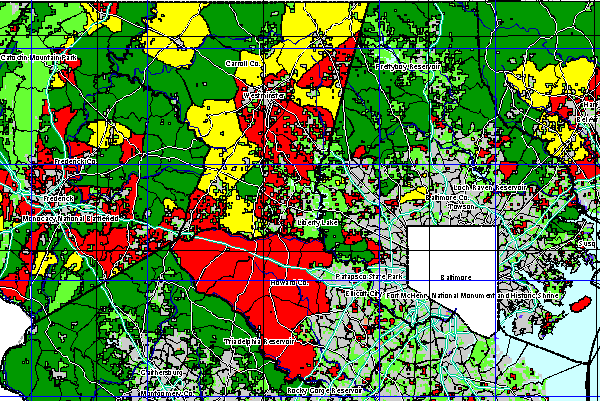
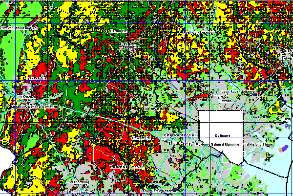
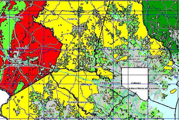
5.1.2 Maryland Statewide
The objectives for the Maryland Landuse, Zoning, and Farmland Protection Map are the same as
at the county level, at a larger geographic extent. (See Image 2, Detail, Maryland Landuse,
Zoning, and Farmland Protection.) To maintain map readability at a smaller map scale, a
sequence of feature selection and generalization took place for landuse, zoning, protection, public
lands and streams.
Image 2, Detail, Maryland Landuse, Zoning and Farmland Protection
As discussed in Section 4 Data Manipulation and Preprocessing, Landuse was generalized to a
minimum mapping unit of 62,500 square meters (6.25 hectares, 15.44 acres, or 672,744 square
feet). This technique eliminates landuse polygons smaller than 62,500 square meters, and
replaces them with the majority landcover within a given 6.25 hectare area. This was conducted
to avoid unnecessary map complexity, and to merge county level databases into a single
statewide database. Landuse vector databases for each county were rasterized at 250 meter cell
size and subsequently merged to a full Maryland statewide landuse GRID database
(MD_LU_GRD). A majority filter function was passed over the grid to eliminate nodata gaps
between counties. The resulting GRID database was converted to a polygon database (MD_LU)
for cartographic display. The same six landuse classes are symbolized : built-up/developed,
agricultural landuse, forested landuse, other landuse, water, and wetlands.
Maryland statewide farmland protection in the form of state easements, county TDRs and PDRs
and private conservation areas were generalized into point or dot symbols representing the
centroid of the protected area. The centroid of each protection for each county was identified and
stored as a point ArcInfo coverage. Maryland Agricultural Easements are shown as red
dots. Maryland Agriculture Preservation Districts are shown as orange dots and Maryland
Environmental Trust areas are yellow dots. TDRs and PDRs are blue and purple dots,
respectively. Privately-owned protected lands smaller than 6,250,000 square meters (625
hectares, or 1,544 acres) are green dots. Privately-owned protected lands larger than 6,250,000
square meters are represented as open green border polygons. (5)
County zoning density requirements for agricultural lands are also portrayed on the statewide
map. The zoning density requirements, which are the number of acres of land required per
household unit in agriculturally zoned areas, are categorized into low, medium and high
agriculture zoning protection and are represented in green, yellow, and red diagonal hatch marks
respectively. Low zoning protection requires less than 10 acres per unit density. Moderate zoning
protection requires 10 to less than 20 acres per unit density. High zoning protection requires
more than 20 acres per unit density. Zoning density was stored as a grid, and merged with a
zoning grid to extract only those areas zoned for agriculture. The density requirements are
represented on the map only on areas zoned for agricultural landuse. (6)
Each Maryland county was assigned a single agricultural zoning density requirement as indicated
in the following table provided by the Maryland Office of Planning :
Table 2. Average Maryland County Agricultural Zoning Density Requirements
| County | Agricultural Zoning Density (Units/Acre) |
| Allegany | 1/25 |
| Anne Arundel | 1/20 |
| Baltimore County | 1/50 |
| Calvert | 1/5 |
| Caroline | 1/20 |
| Carroll | 1/20 |
| Cecil | 1/6 |
| Charles | 1/3 |
| Dorchester | 1/1 |
| Frederick | 1/25 |
| Garrett | 1/25 |
| Harford | 1/10 |
| Howard | 1/4 |
| Kent | 1/20 |
| Montgomery | 1/25 |
| Prince George's | 1/5 |
| Queen Anne's | 1/10 |
| Saint Mary's | 1/3 |
| Somerset | 1/1 |
| Talbot | 1/25 |
| Washington | 1/1 |
| Wicomico | 1/5 |
| Worcester | 1/1 |
Maryland statewide zoning density is stored as an ArcInfo polygon coverage MD_Z_DENS_P.
Publicly-owned lands, which consist of Federal and DNR properties, and county parks, were rasterized and merged into a single statewide grid with a 250 meter cell size. The resulting grid was then converted into a polygon coverage (MD_PUB_P) for cartographic representation. Only those public lands whose areas are greater than 6,250,000 square meters (625 hectares, or 1,544 acres) are shown. The Maryland Landuse, Zoning, and Farmland Protection map depicts publicly owned lands as open thick black border polygons.
The road network and county boundaries are represented statewide from the same data used at
the county level. All county road and county boundary databases were joined into a single
statewide arc coverage (MD_RD). State boundaries from the ARC/USA database were used to
symbolize regional state boundaries. The same source was used for major rivers/streams.
Return to Table of Contents
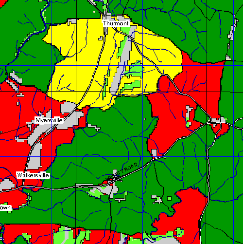
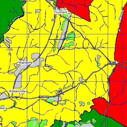
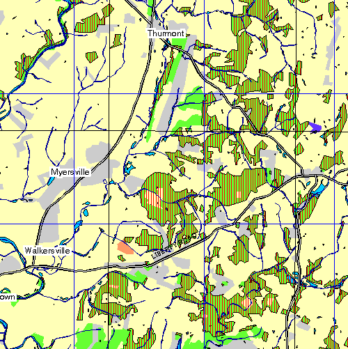
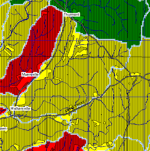
5.2 Analysis Procedures for Projected Development Pressure on Farmland Maps 5.2.1 Frederick County
The Frederick County Projected Development Pressure on Farmland 1995-2020 map is an effort
to represent the spatial distribution and pattern of development pressures on farmland within
Frederick County, Maryland. It focuses on the threat of development pressure on farmland
through the translation of population migration and expansion into household increase.
Conceptually, two basic analytical steps are applied to map development pressure on farmland.
First, the potential buildout, or the number of acres potentially converted to built-up landuse is
identified for an area. Then, potential buildout is then divided by the number of acres of farmland
within that same area to show development pressure expressed as a ratio.
Potential buildout is modeled by Transportation Analysis Zone (TAZ) or Election District (ED)
by multiplying the forecasted increase in the number of households (provided by the Maryland
Office of Planning) from 1995 - 2020 by the county average parcel size in acres for residential
agriculture parcels. The TAZ and EDs are the smallest enumeration areas available statewide
showing current household increase forecasts. Potential buildout shows the number of acres of
farmland which could potentially be converted to built-up landuse within a given TAZ or ED.
Potential Buildout = household increase 1995 - 2020 x county average residential agriculture
parcel size in acres
Image 3, Detail, Frederick County Projected Development Pressure on Farmland 1995 - 2020
Development pressure is modeled by dividing TAZ or ED potential buildout by the number of
acres of farmland (areas zoned for agriculture or areas with agricultural landuse) within a given
TAZ or ED. It shows the ratio, then, of potential farmland conversion to the number of acres of
farmland available.
![]()
This model for development pressure is implemented using ArcInfo GRID GIS software. To
map potential buildout, two basic information surfaces are required. First, TAZ/ED forecast
household increase values from 1995-2020 are gridded at a cell size of 100 meters. (8) Next, the
county average size for all residential agriculture parcels (in 1993) is rasterized to a grid surface.
The surface represents county by county the average size for residential agriculture parcels. In the
case of Frederick County, the average parcel size used was 12.78 acres. The grid representing
household increase per TAZ/ED is multiplied by the grid representing the residential agriculture
parcel size to produce a new grid showing potential buildout of farmland per TAZ/ED.
To map development pressure, two additional basic information surfaces were produced. First,
landcover and landuse zoning were rasterized at a cell size of 100 meters. Next, based on zoning
and landuse grids, the area in acres of lands zoned for farmland or lands used for farming was
calculated for each TAZ/ED and rasterized. The result is a TAZ/ED grid surface showing the
area in acres of farmland per TAZ/ED. The potential buildout surface is divided by the resulting
grid to produce a continuous surface of development pressure. The development pressure surface
is then screened to show development pressure only on those areas zoned for farmland or lands
used for farming.
Development pressure is then simplified into low, medium, and high range categories. The
categories, or bins of development pressure are stored as a polygon coverage (FR_DPRESS_P).
Low development pressure areas have from 0 to less than 0.5 buildout to farmland acres per
TAZ/ED ratios. Low development pressure is represented in dark green areas on the Frederick
County Projected Development Pressure on Farmland 1995-2020 map. Moderate development
pressure areas have from 0.5 to less than 0.75 buildout to farmland acres per TAZ/ED ratios.
These areas are symbolized as deep yellow areas on the Frederick County Projected
Development Pressure on Farmland 1995-2020 map. High development pressure areas have
greater than 0.75 buildout to farmland acres per TAZ/ED ratios.
Selected features found on the Frederick County Landuse, Zoning, and Farmland Protection map
are portrayed on the Frederick County Projected Development Pressure on Farmland 1995-2020
map to provide a context for development pressure and protection. TAZ/ED boundaries are also
portrayed on the map to depict the original enumeration units for the analysis.
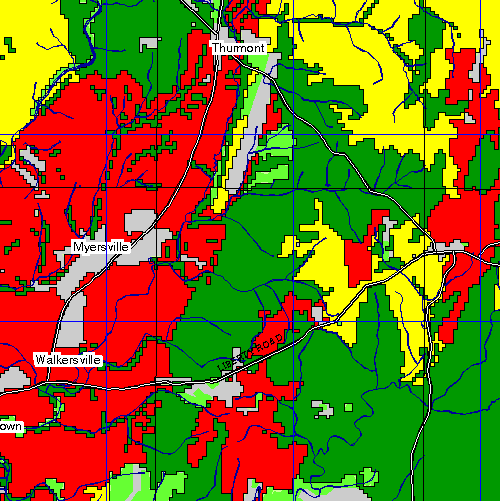
5.2.2 Maryland Statewide
Image 4, Detail, Maryland Projected Development Pressure on Farmland, 1995 - 2020
The conceptual process for deriving development pressure for Maryland statewide is identical to the
process used at the county level. Farmland potential buildout is divided by the acreage of
farmland per unit area to generate development pressure on farmland across Maryland.
The model is implemented statewide by first rasterizing forecast household increase 1995 - 2020
per TAZ/ED for each county. Subsequently each county grid is merged to produce a statewide
surface of household increase. The statewide household increase grid is multiplied by a grid
representing each county's average residential parcel size in acres. Table 3, Maryland Average
Acres per Parcel for Residential Agriculture (With and Without Improvements) lists the county
average parcel sizes used in the Maryland statewide model. The result is a statewide farmland
buildout potential surface.
Table 3, Maryland Average Acres per Parcel for Residential Agriculture
(With and Without Improvements)
| County | County Average Acres for Residential Agriculture Parcel |
| Allegany County | 9.14 |
| Anne Arundel | 8.88 |
| Baltimore County | 8.90 |
| Calvert County | 9.54 |
| Caroline County | 12.30 |
| Carroll County | 8.79 |
| Cecil County | 9.63 |
| Charles County | 14.06 |
| Dorchester County | 10.47 |
| Frederick County | 12.78 |
| Garrett County | 10.78 |
| Harford County | 10.17 |
| Howard County | 12.66 |
| Kent County | 11.38 |
| Montgomery County | 8.21 |
| Prince George's County | 0.59 |
| Queen Anne's County | 17.03 |
| Saint Mary's County | 11.37 |
| Somerset County | 9.63 |
| Talbot County | 10.36 |
| Washington County | 10.46 |
| Wicomico County | 10.71 |
| Worcester County | 10.80 |
The statewide buildout potential surface is then divided by a gridded surface representing the
statewide area in acres of farmland (areas zoned for farmland or areas with agricultural landuse)
per TAZ/ED. The result is a continuous surface of development pressure per TAZ/ED. This
surface is then screened to areas of farmland and generalized into low, medium, and high
development pressure categories. The bins used match the county development pressure
categories. Low pressure ranges from 0 to less than 0.5 buildout to farmland acres per TAZ/ED.
Moderate pressure ranges from 0.5 to less than 0.75 buildout to farmland acres per TAZ/ED.
High development pressure is 0.75 or greater buildout to farmland acres per TAZ/ED. The
resulting statewide development pressure categories grid is polygonized (MD_DPRESS_P) for
cartographic display. Low pressure is symbolized in green, moderate pressure appears in yellow,
and high development pressure appears in red.
Selected features found on the Maryland Landuse, Zoning, and Farmland Protection map are
portrayed on the Maryland Projected Development Pressure on Farmland 1995-2020 map to
contextualize development pressure and farmland protection. TAZ/ED boundaries are also
portrayed on the map to depict the original enumeration units for the analysis.
Return to Table of Contents
5.2.3 Alternate Methodological Approaches for Projected Development Pressure on Farmland
Map
Three basic alternate approaches for modeling development pressure were identified and tested for this concept of operations document. In general terms, the alternates implemented resulted in development pressure maps that reflect modeling assumptions which are significantly more complicated than the approach discussed above. Each approach modeled development pressure based on household increase, but modified household increase by a number of geophysical, distance, and zoning parameters.
The first alternate approach considered was an implementation of development pressure at the cellular, rather than the TAZ/ED level. While this approach may have implied a spatial precision greater than the TAZ/ED level, it was rejected because of the significant fracturing of development pressure patterns in small areas. Moreover, forecast household increase projections are available statewide only at the TAZ/ED level. Cell-level modeling makes an undesirable assumption of spatial accuracy at a level lower than is appropriate for the available household increase information.
The second approach to modeling development pressure accounted for the impact of transportation infrastructure in producing corridor-based development pressure. It also modeled development pressure at the cellular level. Analysis of historical landcover change data for the Baltimore-Washington area from 1966 to 1982 revealed that 95% of all change from non-urban to urban landcover occurred within only ~2.1 miles (~3.4 km) of major transportation arterials. (9) Development pressure within the Baltimore-Washington area may be characterized as transportation- infrastructure guided. Landcover proximity to major arterials greatly increased the probability of landcover conversion to built-up. The alternate development pressure modeling approach incorporated this information by increasing development pressure by a given factor for farmlands within 2.1 miles of a major arterial. As farmland distance from major arterials increased, development pressure decreased proportionally.
This modeling practice, while common in development pressure modeling, was rejected because of concerns over unnecessary complexity and the potential for colinearity, or redundant interaction, between a distance decay-driven development pressure model and distance decay modeling factors applied in strategic farmland and farmland viability models.
A third modeling approach for development pressure was the incorporation of terrain and zoning information to modify development pressure. The approach accounts for the impact of zoning and terrain slope to assess the potential suitability of land for development. The approach reduces development pressure in the form of household increase on areas with slope that is too high to be developed or built up, while increasing pressure on areas with low slope. Moreover, landuse zoning modifies development pressure under the model downward in areas zoned for conservation, while pushing pressure upward in areas zoned for development or in areas with sewer service districts.
Since the significance and magnitude of pressure increase or decrease for different zoning areas relies on explicit assumptions which may be considered qualitative, rather than quantitative, the incorporation of zoning and sewer service areas into the model was rejected. The incorporation of slope information was rejected since it would require modeling at the cellular level, rather than the TAZ/ED level.
Lastly, modeling of development pressure based on the nominal county zoning density for
agriculture, rather than parcel size information was implemented to generate the buildout
component of the model. This alternate approach is an additional attempt to incorporate zoning
requirements. The model was rejected by the Farms for the Future Board in favor of the parcel
size-based model. Concerns over the long term viability and accuracy of the zoning, in
comparison with the effective zoning density were raised. Efforts are underway to implement a
development pressure model based on the effective, or in-practice county zoning density
requirements for agriculture.
Return to Table of Contents
5.3 Analysis Procedures for Farmland Agricultural Significance
It was stated earlier that this concept of operations document and the Chesapeake Farms for the
Future Mapping Project approaches the issue of mapping farmland significance through multiple
themes. Soil- and non-soil based productivity, as well as non-agricultural features on farmland,
are mapped to capture the agricultural significance of the Chesapeake landscape.
Return to Table of Contents
5.3.1 Analysis Procedures for Farmland with Significant Agricultural Features (Based on Soil
Productivity) Maps 5.3.1.1 Frederick County
The Frederick County Farmland with Significant Agricultural Features (Based on Soil
Productivity) map represents agriculturally significant farmlands within Frederick County from a
soil productivity standpoint. The map identifies areas of low, moderate and high soil-based
farmland productivity.
Image 5, Detail, Frederick County Farmland with Significant Agricultural Features (Based on Soil Productivity)
Conceptually, the model combines soil yield information on several crop types from State Soil
Geographic (STATSGO) Data Base soil units with generalized Maryland Natural Soils Groups
ratings for soil agricultural productivity. This combination produces soil productivity performance ratings on
farmland areas. Soil yield information, measured as an average yield potential for several crop
types appropriate to Maryland, are multiplied by a weighting factor based on the Maryland
Natural Soils Groups ratings information. Areas with better Natural Soils Group ratings receive
higher productivity multiplier factors, while areas with lower Natural Soils Groups ratings
receive lower productivity multipliers. Soil-based productivity may be symbolized in the
following conceptual formula:
Soil-Based Productivity = Average Soil Crop Yield x Soil Productivity Ratings
The soil productivity model was implemented using ArcInfo GRID. Soil yield information
was processed using STATSGO soil units, provided by the US Department of Agriculture Soil
Conservation Service and National Soil Survey Center. A soil-based yield value for each soil unit
was derived by multiplying the average soil unit yield in bushels for corn, wheat, soy, and oats
times the average soil unit yield in tons of grass-legume hay, corn silage, and alfalfa hay. The
result is an aggregated average soil crop yield grid.
A grid showing ratings for soil productivity was next generated from the Generalized Maryland
Natural Soils Groups database provided by the Maryland Office of Planning. The Generalized
Maryland Natural Soils Groups database represents areas of soil productivity characterized as
prime, productive, or other productivity. A grid was produced for Frederick County which placed
rating values for soil productivity based on the Soils Groups. Areas with prime productivity were
given a weighting factor of 3. Areas with productive ratings were assigned a factor of 2. Areas
with the 'other' productivity were assigned a 1. The result was a gridded surface representing soil
productivity ratings.
The next analytic step in the model is the multiplication of the aggregated average soil crop yield
grid by the soil productivity ratings grid. The output is then screened to farmland areas (areas
zoned for agriculture or of agriculture landuse).This step produces a grid surface showing the
interaction of soil yield performance and soil productivity ratings.
The resulting grid is categorized into low, medium, and high soil-based productivity bins. The
soil productivity category ranges were chosen based on "natural breaks" in the gridded data. The
categories minimize the variance in productivity within the bins, while maximizing the
productivity variance between the bins. The grid is converted into a polygon coverage
(FR_PROD_P) for cartographic display. Low soil-based productivity ranges from 0 to less than
970, and is symbolized as dark green areas on the Frederick County Farmland with Significant
Agricultural Features (Based on Soil Productivity) map. Moderate soil-based productivity ranges
from 970 to less than 1600 and is symbolized as deep yellow areas on the county map. High
soil-based productivity ranges from 1600 to a maximum productivity of 2,353. High soil-based
productivity areas are shown in red on the soil-based productivity map.
Selected features included on the Frederick County Landuse, Zoning, and Farmland Protection
map are portrayed on the Frederick County Farmland with Significant Agricultural Features
(Based on Soil Productivity) map as a reference for the interaction of soil-based farmland
productivity and farmland protection.
5.3.1.2 Maryland Statewide
Image 6, Detail, Maryland Farmland With Significant Agricultural Features (Based on Soil Productivity)
The analytic concepts and implementation for modeling Maryland statewide farmland with
significant agricultural features based on soil productivity are based on the county-level
approach. Image 6, Maryland Farmland with Significant Agricultural Features (Based on Soil
Productivity) portrays Maryland statewide soil productivity on farmland. The additional step of
rasterizing and merging each county Maryland Natural Soils Group ratings database to a single
statewide grid at a cell size of 500 meters (25 hectares, or 61.77 acres) was taken. The same
coding scheme for the county level was applied statewide. A rating score of 3 applies to areas
with prime productivity. A 2 is assigned to areas with the productive rating, and areas with 'other'
productivity are assigned a 1.
The Maryland Statewide STATSGO soil yield ratings (which are the average yield in corn,
wheat, soy, and oats times the average soil unit yield in tons of grass-legume hay, corn silage,
and alfalfa hay) were also rasterized at 500 meter cell size (25 hectares, or 61.77 acres). The
resulting grid is multiplied by the statewide soil productivity ratings grid to produce a statewide
soil productivity grid. The grid is screened to farmlands and categorized into low, medium, and
high productivity bins. The category ranges are identical to the natural breaks bins applied at the
county level. Low soil-based productivity ranges from 0 to less than 970, moderate soil-based
productivity ranges from 970 to less than 1600, and high soil-based productivity ranges from
1600 to a maximum productivity of 2,353. The resulting grid is polygonized into an ArcInfo
polygon coverage (MD_PROD_P). Low, moderate, and high soil productivity are portrayed as
deep green, yellow, and red areas respectively on the Maryland Farmland with Significant
Agricultural Features (Based on Soil Productivity) map.
Selected features found on the Maryland Landuse, Zoning, and Farmland Protection map are
portrayed on the Maryland Farmland with Significant Agricultural Features (Based on Soil
Productivity) map to represent soil-based productivity and farmland protection. State and local
farmland protections are simplified into open black circles to avoid cartographic interaction
between protection symbol colors and productivity symbol colors.
An alternate approach to modeling soil-based productivity at the state and county level using a
different crop mix is currently underway. This approach selects yield information for the top four
crop types, based on acreage for each of the six Maryland regions, as defined by the Maryland
Office of Planning. This scenario trades a single, consistent set of crops for crop type mixes that
change from region to region to produce more locally significant productivity results.
Return to Table of Contents
5.3.2 Analysis Procedures for Farmland with Significant Agricultural Features (Based on
non-Soil Productivity) 5.3.2.1 Frederick County
Image 7, Detail, Frederick County Farmland with Significant Agricultural Features (Based on
non-Soil Productivity) is an attempt to map the significance of Chesapeake farmland from a
farmland sales value perspective. The map shows areas of low, medium, and high farmland sales
per acre of farmland along with basic reference information provided on the County Landuse,
Zoning, and Protection map.
Conceptually, the non-soil productivity map shows the weighted total value of agricultural
products sold per farmland acre within a given farmland area. The model is implemented through
ArcInfo GRID.
Image 7, Detail, Frederick County Farmland with Significant Agricultural Freatures (Based on non-Soil Productivity)
The only consistent source of sub-county level agriculture sales data Maryland statewide is found
in the U.S. Census of Agriculture 1992 ZIP Code Farm Counts database. The database is a count,
by ZIP code of the total number of farms meeting varying agriculture census criteria. In the case
of total value of agricultural sales, the U.S. Census of Agriculture 1992 ZIP Code Farm Counts
database records the total number of farms whose sales are greater in value than $1,000 per year
in 1992.
To derive subcounty level agricultural sales information, the ZIP code farm counts serve as a
weighting value on county-level total sale value of agricultural products for 1992. The ZIP code
proportion of total farms is calculated and gridded. The resulting grid shows the proportion of
total farms each ZIP code contains of the Frederick County total number of farms. This
proportion surface is then multiplied by the total value of agricultural products sold for all of
Frederick County in 1992 to derive a weighted total value of agricultural products sold by ZIP
code. The conceptual formula for ZIP weighted county total value of agricultural products sold
is:

The ZIP weighted county total value of agricultural products sold is then divided by the total acres of farmland per ZIP code (derived from Maryland Office of Planning landuse and zoning data) to generate a sales density surface. County nonsoil productivity is defined as ZIP code level total sales per farmland acre :

Non-soil productivity is screened to farmland (acres zoned for agriculture or areas with
agriculture landuse) and then categorized into low, medium, and high non-soil productivity bins.
Low non-soil productivity ranges from $0 to less than $325 total agricultural product sales value
per acre. Moderate non-soil productivity ranges from $325 to less than $487 total agricultural
product sales value per acre. High non-soil productivity ranges from $487 to a maximum total
agricultural product sales value per acre of $6,124. The category ranges are based on natural
breaks within the data. The bins are designed to minimize variance within the groups and
maximize variance between the groups. Low non-soil productivity is depicted in dark green,
while moderate non-soil productivity is portrayed in yellow and high non-soil productivity is
portrayed in red.
Selected Frederick County Landuse, Zoning, and Farmland Protection map features are also
included on the Frederick County Farmland with Significant Agricultural Features (Based on
non-Soil Productivity) map .
Return to Table of Contents
5.3.2.2 Maryland Statewide
Image 8, Detail, Maryland Farmland with Significant Agricultural Features (Based on non-Soil Productivity)
The conceptual approach to the Maryland Farmland with Significant Agricultural Features
(Based on non-Soil Productivity) map differs from the county counterpart map in terms of the
enumeration units used. The concept for the map is a choropleth design showing at the county
level the total dollar value of agricultural products sold per farmland acre. No interpolation of
sales information is made on the Maryland statewide modeling approach.
The model is implemented by gridding the county total value of all agricultural products sold in
1992 (recorded by the US Census of Agriculture) to a statewide surface with a cell size of 250
meters. The sales surface is then divided by the county total acres in farmland (from the 1992 US
Agriculture Census). The resulting surface is the nonsoil productivity measurement to be
mapped:

Nonsoil productivity is screened to those areas zoned for agriculture or of agricultural landuse.
The resulting grid is categorized using the "natural breaks" method into low, moderate, and high
non-soil productivity categories. The categorized grid is converted to a polygon coverage for
cartographic display (MD_SALES_P).
In the Maryland statewide model, low non-soil productivity ranges from $0 to less than $325
county total value of agricultural products sold per farmland acre in 1992. Low non-soil
productivity is shown in deep green areas. Moderate non-soil productivity ranges from $325 to
less than $487 county total sales value per farmland acre in 1992. Moderate productivity is
symbolized in deep yellow areas. High non-soil productivity ranges from $487 to a maximum of
$2,958 county total sales value per farmland acre. Areas in deep red represent highest farmland
non-soil productivity.
The Maryland Farmland with Significant Agricultural Features (Based on non-Soil Productivity)
map also portrays selected features found on the Maryland Landuse, Zoning, and Farmland
Protection map.
Return to Table of Contents
5.4 Analysis Procedures for Farmland with Significant Non-Agricultural Features
(Environmental, Cultural, and Historic)
This concept of operations also assesses the value of Chesapeake Farmlands from a
nonagricultural standpoint. Maps representing the distribution and pattern of environmental,
cultural, and historic features on Chesapeake farmland were produced.
Return to Table of Contents
5.4.1 Frederick County
Image 9, Detail, Frederick County Farmland with Significant Non-Agricultural Features (Environmental, Cultural, and Historic)(Draft)
Conceptually, the Frederick County Farmland with Significant Non-Agricultural Features (Environmental, Cultural, and Historic) map is an overlay map. It records the location and extent of cultural, historical, and environmental features located on Frederick County farmlands.
The environmental component of the map currently consists of forested areas zoned for agriculture, species habitat, and wetlands on farmlands.
Sensitive forested lands zoned for agriculture were selected from landuse and zoning coverages provided by the Maryland Office of Planning. The US Fish & Wildlife National Wetlands Inventory (NWI) polygon coverage, provided Maryland statewide by the Maryland DNR, is screened by size to call out significant wetlands. Significant wetlands are defined as wetlands on farmland with an area greater than 7,500 square meters (1.85 acres).
Basemap features from the Frederick County Landuse, Zoning and Farmland Protection map are included to provide spatial context for non-agricultural sensitivity.
When data collection is completed, the map will show known zones of endangered species
habitat, forest interior habitat, forest legacy sites, waterfowl staging areas, waterfowl nesting
areas, and wetlands and areas of Critical State Concern (provided by the Maryland DNR). The
map will also portray archeological sites, historic sites, and historic property locations (provided
by the Maryland Historic Trust) on farmlands.
Return to Table of Contents
5.4.2 Maryland Statewide
Image 10, Detail, Maryland Farmland with Significant Non-Agricultural Features (Environmental, Cultural, and Historic) (Draft)
The Maryland Farmland with Significant Non-Agricultural Features (Environmental, Cultural, and Historic) map follows design concepts similar to those described for the Frederick County map. Information components for environmental, historic and cultural farmland significance are combined through overlay to produce a composite map showing the distribution and pattern of non-agricultural farmland significance. Features from the county level map are also portrayed at the state level.
Wetlands from the US Geological Survey Land Use and Land Cover database were extracted and combined with wetland areas from the Maryland Office of Planning composite databases to produce a comprehensive statewide wetlands base. NWI wetlands were not used at the state level. In addition, farmlands within 1,000 feet of Chesapeake Shoreline have been highlighted to emphasize the pattern of farmlands within sensitive shoreline areas.
As with the county map, once data collection is completed, the map will portray a number of
additional geographic themes highlighting the environmental, cultural, and historic significance
of farmland.
Return to Table of Contents
5.5 Analysis Procedures for Projected Subwatershed Surface Imperviousness Increase 1995 -
2020 Map
GIS analytic tools were applied to model expected surface imperviousness increase at the
subwatershed level. The maps produced serve as indicators of the threat to water quality through
increasing surface imperviousness on farmland.
Return to Table of Contents
5.5.1 Frederick County
Image 11, Detail, Frederick County Projected Average Subwatershed Surface Imperviousness Increase 1995-2020
Image 11 shows a detail view of the Frederick County Projected Average Subwatershed Surface
Imperviousness Increase 1995 - 2020 map. The map shows projected surface imperviousness
increase by sub watershed for 1995 through 2020. It is an effort to emphasize the relationship of
farmlands and water quality. It attempts to draw the impact of spreading landcover
imperviousness on water quality to farmland protection planning.
Conceptually, the model measures surface imperviousness increase as the product of household
increase per acre and the average imperviousness increase expected per household unit increase.
The model concept, expressed as a formula, is:
Surface Imperviousness Cover Increase = Increase in Households per Acre x Expected Increase
in Imperviousness per Household Increase Per Acre
The model is implemented using ArcInfo GRID at a cell size of 100 meters. A number of
assumptions and constraints on the model have been made. The basic modeling process is to first
produce a raster surface of forecast household increase per acre by Transportation Analysis Zone
(TAZ) or Election District (ED). The surface is then multiplied by the expected increase in
imperviousness per household increase per acre per TAZ or ED. The TAZ/ED expected
imperviousness increase is then adjusted to subwatersheds through averaging. Subwatershed
boundaries are provided by the Maryland Department of Natural Resources. The resulting surface
is simplified into low, medium and high categories of increase.
The increase per acre by TAZ or ED was derived from household increase forecasts provided by
the Maryland Office of Planning. The household increase per acre was adjusted to permit an
increase in households only up to the average zoning density requirement of agriculture for each
county. (See Table 2, Average Maryland County Agricultural Zoning Density Requirements, for
a list of the average zoning density requirements used for each county). Therefore, any increase
in households beyond that permitted under the zoning density requirement is removed from
consideration in the model. This approach assumes both the enforcement of zoning density
requirements and that any household increase in excess of the requirement represents increase in
areas already built-up.
The expected increase in imperviousness per household increase per acre per TAZ or ED was
derived from a base rule provided by the Maryland Office of Planning. The guideline used is that
at a zoning density of one household unit per 20 acres, 12% of landcover is expected to be
impervious. Translated into expected increase in imperviousness per household increase per acre
per TAZ or ED, the imperviousness cover is a constant scalar of 2.4. Expressed algebraically,

Therefore,
TAZ/ED surface impervious increase (percent) = TAZ/ED adjusted increase in households per
acre (up to the zoning density requirement) x 2.4
The resulting TAZ/ED surface imperviousness increase GRID is then overlaid with a gridded
subwatershed surface. The average percent surface imperviousness increase for subwatersheds is
then calculated (FR_IMPERVM). The imperviousness increase is then simplified into low,
medium, and high surface imperviousness increase categories as shown in the following Table 4:
Table 4 Subwatershed Average Percent Surface Imperviousness Increase Category Ranges
| Imperviousness Increase | Imperviousness Increase Range |
| Low | 0 < 5% |
| Moderate | 5% < 8% |
| High | 8% + |
The result is a grid of low, moderate and high surface imperviousness increase for subwatersheds
(FR_IMPERV_BIN). The grid is converted to a polygon for cartographic display
(FR_IMPERV_P).
The features included on the Frederick County Landuse, Zoning, and Farmland Protection map
are portrayed on the Frederick County Projected Average Subwatershed Surface Imperviousness
Increase 1995 - 2020 map as a reference for the interaction of surface imperviousness increase
and farmland protection. Since landuse information is concealed by the subwatershed
information, farmlands (areas zoned for agriculture or of agriculture landuse) have been called
out with a hatch pattern overlaying the subwatersheds. Water landcover was also portrayed for
the Chesapeake bay.
Return to Table of Contents
5.5.2 Maryland Statewide
Image 12, Detail, Maryland Projected Average Subwatershed Surface Imperviousness Increase 1995-2020
Image 12, Detail, Maryland Projected Average Subwatershed Surface Imperviousness Increase
1995 - 2020 shows the increase of surface imperviousness Maryland statewide.
The mapping methodology invokes the same concepts and operations used at the county level
design. First, a statewide 250 meter cell-size (15.44 acres) raster surface of forecast household
increase per acre by TAZ/ED is produced. The surface is multiplied by the expected increase in
imperviousness per household increase per acre per TAZ or ED. The TAZ/ED expected
imperviousness increase is then adjusted to subwatersheds through averaging. The resulting
surface is simplified into low, medium and high categories of imperviousness increase. (See
Table 4, above, for a breakdown of the category information.) The resulting grid (MD_SW_IMP)
is converted into polygons for cartographic display (MD_SW_IMP_P).
Maryland Landuse, Zoning, and Farmland Protection map features are also incorporated with the
Maryland Projected Average Subwatershed Surface Imperviousness Increase 1995 - 2020 map.
Farmlands have been represented with an overlaid hatch pattern.
Return to Table of Contents
6.0 Quantitative Output Analysis Products
This document presents a set of representative acreage summary tables and charts as examples of
the analytical capabilities of Geographic Information Systems to engineer information useful in
building knowledge for farmland protection within the Chesapeake Bay.
Return to Table of Contents
6.1 Acreage Summary Tables Samples
A series of data tables was produced representing acreage conditions of farmland in terms of development pressure, agriculture productivity, and development pressure on farmland productivity. Summary frequency tables were produced for the County, Regional, Watershed and Statewide levels for Maryland.
The County, Regional, Watershed, and Statewide Farmland Acreage Summary Table shows the total acreage of farmland (lands of agriculture use or zoned for agriculture) for each county, six Maryland Regions, the Chesapeake Bay watershed area of Maryland, and Maryland statewide. The table also shows each geographic subarea's proportion of the total Maryland farmland.
The table was produced using information derived through raster-based analysis in ArcInfo GRID. Combined farmlands and enumeration unit geography were rasterized Maryland statewide at a cell size of 250 meters. Farmland acreage frequencies were calculated using MICROSOFT EXCEL. The minimum mapping unit for calculating acreage is 62,500 square meters, or 15.44 acres. All of the summary tables presented in the concept of operations document follow these computational parameters.
Maryland Regions are functional groupings of counties as defined by the Maryland Office of
Planning. Table 5, Maryland Regions Counties List shows the composition of each of the six
Maryland Regions.
Table 5, Maryland Regions Counties List
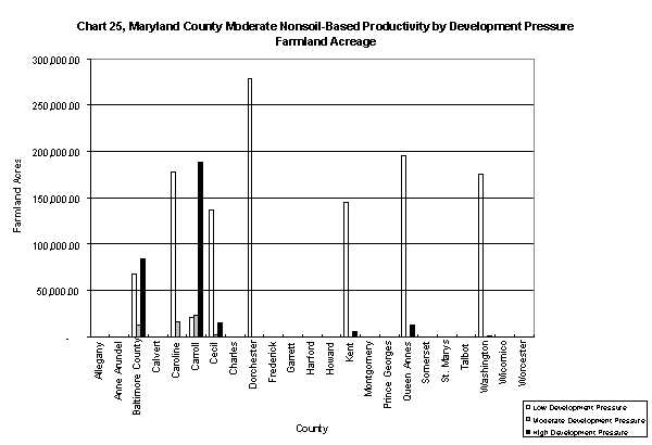
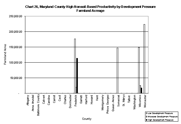
Development Pressure on Farmland is tabulated on the Maryland Development Pressure on Farmland County Watershed Acreage Summary table. The table was produced based on a raster cell size of 250 meters. The table shows the breakdown of low, moderate, and high development pressure on farmland for each county under the "% of Total County Farmland Acres" column. The "% of Maryland Total Acres (All Farmland)" column shows the county's share of all Maryland Farmland. The last column, "% of Maryland Total (by Pressure Category) shows each county's share of farmland by development pressure level. The table also presents development pressure summary information for the Chesapeake Bay watershed area of Maryland and Maryland statewide (the "% of Maryland Total Acres (All Farmland)" column). Similar information is summarized by the six Maryland Regions in the Maryland Development Pressure by Region Summary Table.
The Maryland Soil-Based Productivity County, Watershed, and Statewide Farmland Acreage is a
tabulation of farmland significance acreage from a soil-based perspective. The table portrays
each County's proportion of low, moderate and high soil-based productivity. It also shows each
county's share of Maryland statewide soil-based farmland productivity, along with each county's
share by soil-based productivity level. The Maryland Regional Soil-Based Productivity Farmland
Acreage Summary Table computes similar information on a regional basis. It summarizes the
Maryland regional acreage of low, moderate, and high soil-based farmland productivity.
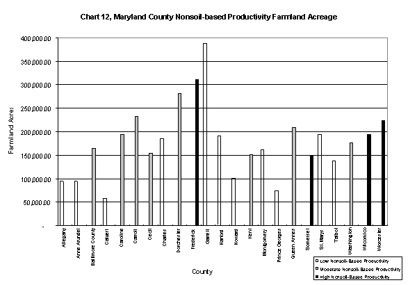
The Maryland Non-soil Based Productivity County, Watershed, and Statewide Farmland Acreage
summarizes Maryland county-level non-soil based productivity. Each county has a single
non-soil productivity rating, and the table portrays each county's share of Maryland total
farmland and each county's share by nonsoil-based productivity level. The non-soil based
productivity is further synthesized by Maryland Regions in the Maryland Regional
Nonsoil-Based Productivity Farmland Acreage Summary Table.
The Maryland Development Pressure on Farmland Soil-Based Productivity by County,
Watershed, and Statewide Farmland Acreage table synthesizes the distribution of low, moderate,
and high development pressure on low, moderate and high soil-based farmland productivity. The
Columns "Soil Productivity" and "Development Pressure" assess each county's level of soil
productivity and development pressure respectively. The column "% of Total County Farmland
Acres" reveals the breakdown by County of development pressure by soil-based productivity.
The table also shows each soil-productivity by development pressure combination share of
Maryland total farmland acres. The "% of Maryland Total (by Combined Productivity & Pressure
Category)" column in the table shows each county's share of a given soil-productivity and
development pressure combination. The Maryland Regional Development Pressure on Soil-based
Productivity Farmland Acreage Summary Table shows similar information aggregated to the
Maryland Regional level.
The Maryland Development Pressure on Nonsoil-based Productivity, County, Watershed, and
Statewide Farmland Acreage Summary Table, assesses development pressure on non-soil based
productivity. For each county, the county's breakdown of development pressure by non-soil based
productivity is reported in the "% of Total County Farmland Acres" column. The Maryland
Regional Development Pressure on Nonsoil-based Productivity Farmland Acreage Summary
Table presents similar information on a Maryland Regional basis.
Return to Table of Contents
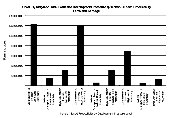
6.2 Acreage Summary Graphs
The information developed by tabulation in the above tables may also be presented in a graphic
form. MICROSOFT EXCEL was used to produce bar charts showing acreage summary
information for farmland, development pressure, soil-based productivity, nonsoil-based
productivity, development pressure on soil-based productivity, and development pressure on
nonsoil-based productivity. The charts are based on information presented in the tables described
in the previous section. Collectively, thirty-one charts portray synthesized Maryland statewide,
Chesapeake Bay Watershed, regional, and county-level information. The selected sample charts
included in this paper are extracted from draft information tables from older models for
development pressure and farmland definitions. Consequently, the charts are intended to
illustrate the charting concepts and do not represent final acreage values for the Farms for the
Future Mapping project.
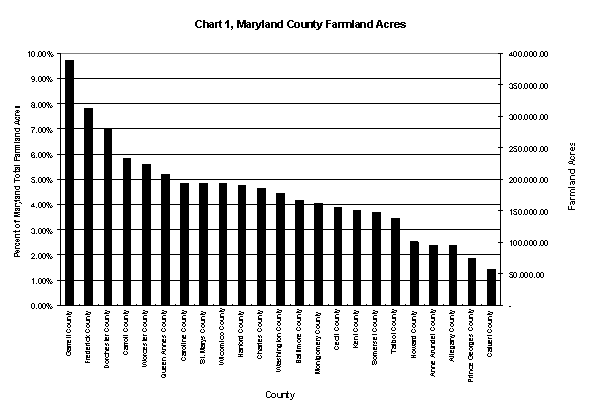
Chart 1, Maryland County Farmland Acres presents the proportion and acreage of the acres of
farmland for each county in Maryland. Chart 2, Maryland Regional Farmland Acres summarizes
the proportion and acreage of the acres of farmland for each Maryland Region. Chart 3, Maryland
Farmland Acres summarizes the total number of acres in farmland for Chesapeake Bay
Watershed Maryland and Maryland Statewide.
Chart 1, Maryland County Farmland Acres
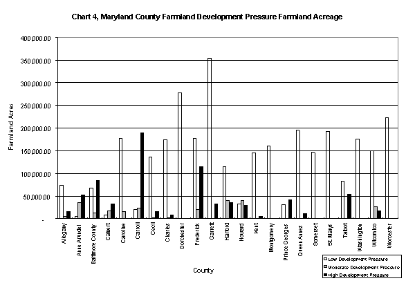
Chart 4, Maryland County Farmland Development Pressure Farmland Acreage portrays the
distribution, in acres, of low, moderate and high development pressure on farmland for each
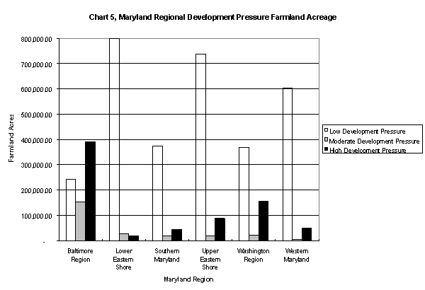
Maryland county. Chart 5, Maryland Regional Development Pressure Farmland Acreage shows
the acreage distribution of low, moderate, and high development pressure on farmland for each of
the six Maryland Regions. Chart 6, Maryland Chesapeake Bay Watershed Development Pressure
on Farmland Acreage shows development pressure categories for the Chesapeake Bay Watershed
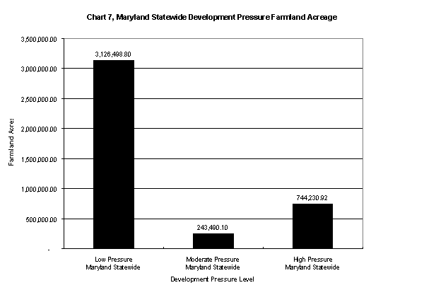
area of Maryland. Chart 7, Maryland Statewide Development Pressure Farmland Acreage depicts
the farmland acreage under low, moderate, and high development pressure for the entire state of
Maryland.
Chart 4, Maryland County Farmland Development Pressure Farmland Acreage
Chart 5, Maryland Regional Development Pressure Farmland Acreage
Chart 7, Maryland Statewide Development Pressure on Farmland Acreage
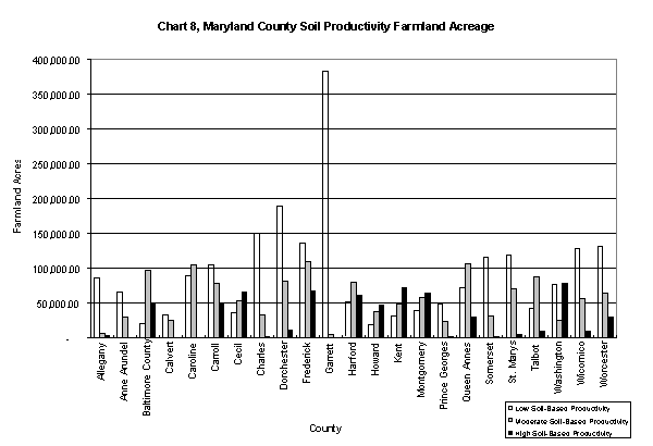
Chart 8, Maryland County Soil Productivity Farmland Acreage shows the distribution of
soil-based farmland productivity (low, moderate, and high) acreage for each Maryland County.
Chart 9, Maryland regional Soi-Based Productivity Farmland Acreage shows low, moderate, and
high soil-based productivity for each Maryland Region. Chart 10, Maryland Chesapeake Bay
Watershed Soil-Based Productivity Farmland Acreage charts out soil-based farmland
productivity for the Chesapeake Bay areas of Maryland. Chart 11, Maryland Statewide
Soil-Based Productivity Farmland Acreage summarizes total soil-based farmland productivity
Maryland Statewide.
Chart 8, Maryland County Soil Productivity Farmland Acreage
Chart 12, Maryland County Nonsoil-based Productivity Farmland Acreage represents the
distribution of county-level acreage of low, moderate, and high non-soil based farmland acres.
Chart 13, Maryland Regional Nonsoil-based Productivity Farmland Acreage shows low,
moderate and high nonsoil-based farmland productivity acreage for each of the six Maryland
regions. Chart 14, Maryland Chesapeake Watershed Nonsoil-based Productivity Farmland
Acreage, shows the distribution of farmland nonsoil-based productivity for the Chesapeake Bay
Watershed area of Maryland. Chart 15, Maryland Statewide Nonsoil-based Productivity
Farmland Acreage summarizes nonsoil productivity to the Maryland statewide level.
Chart 12, Maryland County Nonsoil Based Productivity Farmland Acreage
Chart 16, Maryland County Low Soil-Based Productivity by Development Pressure Farmland
Acreage is an assessment of the distribution development pressure on low soil-based productivity
at the county level. It portrays farmland acres of low soil-based productivity for low, moderate,
and high levels of development pressure for each county. Chart 17, Maryland County Moderate
Soil-Based Productivity by Development Pressure Farmland Acreage assesses the relationship
between moderate soil-based farm productivity and development pressure. Chart 18, Maryland
County High Soil-Based Productivity by Development Pressure Farmland Acreage shows the
interaction of high soil-based farm productivity and development pressure.
Chart 16, Maryland County Low Soil-Based Productivity by Development Pressure Farmland Acreage
Chart 17, Maryland County Moderate Soil-Based Productivity by Development Pressure Farmland Acreage
Chart 18, Maryland County High Soil-Based Productivity by Development Pressure Farmland Acreage
Similar information for the interaction of development pressure on low, moderate, and high
soil-based productivity at the Maryland regional level are portrayed on Charts 19, 20, and 21. In
each case, the acreage of low, moderate and high development pressure on low, moderate and
high soil-based productivity at the Maryland regional level is portrayed.
Chart 22, Maryland Chesapeake Bay Watershed Farmland Development Pressure by Soil-Based
Productivity Farmland Acreage shows the acreage distribution of development pressure on
farmland soil-based productivity at the Chesapeake Bay Watershed level. Chart 23, Maryland
Total Farmland Development Pressure by Soil-Based Productivity Farmland Acreage, shows
each development pressure category by soil-based productivity category for the entire state of
Maryland.
Chart 24, Maryland County Low Nonsoil-Based Productivity by Development Pressure Farmland
Acreage is an examination of the interaction of development pressure with low nonsoil
productivity farmland at the county level. It shows the acreage of low nonsoil-productivity
farmland under low, moderate, and high development pressure for each Maryland county. Chart
25, Maryland County Moderate Nonsoil-Based Productivity by Development Pressure Farmland
Acreage shows the level of development pressure on moderate nonsoil-based farmland
productivity at the county level. Chart 26, Maryland County High Nonsoil-based Productivity by
Development Pressure Farmland Acreage shows the impact of development pressure on high
nonsoil-based farmland productivity for each county.
Chart 24, Maryland County Low Nonsoil-Based Productivity by Development Pressure Farmland Acreage
Chart 25, Maryland County Moderate Nonsoil-Based Productivity by Development Pressure Farmland Acreage
Chart 26, Maryland County High Nonsoil-Based Productivity by Development Pressure Farmland Acreage
Charts 27, 28 and 29 organize development pressure on low, moderate, and high nonsoil-based
productivity into the regional level. They respectively portray for each of Maryland's six regions
the acreage of low, moderate, and high development pressure on low, moderate, and high
nonsoil-based productivity.
Chart 30, Maryland Chesapeake Bay Watershed Farmland Development Pressure by
Nonsoil-Based Productivity Farmland Acreage shows the acreage of each level of development
pressure on farmland nonsoil-based productivity for Chesapeake Bay Watershed Maryland. Chart
31, Maryland Total Farmland Development Pressure by Nonsoil-Based Productivity Farmland
Acreage shows the Maryland statewide total for development pressure on farmland nonsoil-based
productivity.
Chart 31, Maryland Total Farmland Development Pressure by Nonsoil-Based Productivity Farmland Acreage
Return to Table of Contents
7.0 Conclusions
Geographic Information Systems are a viable tool for addressing complex critical questions for farmland protection planning within the Chesapeake Bay. GIS capabilities were applied to produce maps which identify not only the location and extent of farmland protection, but also model development pressure on farmland. GIS tools were also produced which show the relationship between development pressure and farmland productivity from a soil- and nonsoil-based perspective. GIS is the only tool available for quantifying the impact of development pressure on farmland productivity. It is also the only viable tool for producing generations of multiple versions of farmland significance models. The models presented in this paper are the result of several evolutionary changes and improvements to underlying model requirements and assumptions. More changes and improvements are currently underway.
The Chesapeake Farms for the Future Mapping project is near completion. Additional themes which synthesize the complex spatial patterns of development pressure, farmland agricultural and non-agricultural significance, and water quality change for farmlands are to be produced. The resulting synthesized maps will show farmland strategic value for the Chesapeake. These maps will serve to identify the most significant Chesapeake farmlands under threat of ongoing development pressure. The maps will assist planners in identifying, in a meaningful way, areas for well-planned farmland protection.
Return to Table of Contents
Acknowledgments
The author wishes to thank George Maurer of the Chesapeake Bay Foundation and Jill Schwartz
of the American Farmland Trust for their guidance and direction for the Chesapeake Farms for
the Future mapping project. The author wishes to acknowledge the valuable input of former
EarthSat employee Todd Patterson through his review of this paper and technical support.
Thanks also to EarthSat scientists Andy Waxman and Jacques Piou for their technical expertise
and assistance through the life of the project.
Return to Table of Contents
Appendix 1 Metadata Assessment of Fitness for Use of Significant Applied Map Databases
Appendixes
The lineage, positional and attribute accuracy, along with logical consistency and completeness
of spatial data are collectively known as metadata ("quasi-data," or "data about data"). Metadata
is designed to assist users of spatial data in assessing a database's strengths and limitations for
use in a GIS analysis or application. Data lineage is the source, original scale and history of
processing steps in generating map data. Positional accuracy is the horizontal and vertical
positional accuracy of spatial data. Attribute accuracy is the correctness of map theme
characteristics. Data completeness is the extent to which a map database represents all of the
entities it is expected to represent. Logical consistency refers to the correctness of map database
connectedness, adjacency, and the spatial relationships of map data.
This section will identify the basic fitness for use for the significant map databases used in this
concept of operations based on several of these metadata criteria. The following metadata index
table organizes the original data by the source organization provider.
Metadata Index Table
Maryland Office of Planning
County Simplified Land Use, Simplified Zoning, Simplified Sewer Service Areas,
Simplified Soils Suitability, Transportation Analysis Zones (TAZ)/Election Districts (EDs)
composite ArcInfo polygon databases.
The Maryland Office of Planning provided for each Maryland County a composite vector
ArcInfo coverage of landuse/landcover, zoning, sewer service, agricultural soil suitability,
and TAZ/EDs. A total of 23 composite databases, one for each Maryland County was provided.
Lineage:
Simplified Landuse/Landcover
Return to Metadata Index Table
Simplified Zoning was provided by each Maryland County to the MOP which conducted generalization into Residential Development, Other/Commercial Development, Agricultural, Conservation, Wetlands, and Water. Exact source scales for each county are not available.
Return to Metadata Index Table
Simplified Sewer Service Areas were also provided by each county and generalized by the Maryland Office of Planning. The designations were simplified into two classes: (a) all existing or planned sewer service areas, and (b) areas not planned for sewer service. Exact source scales for each county are not available.
Return to Metadata Index Table
Simplified Soil Suitability was generated by the MOP by generalizing the Maryland Natural Soils Groups Ratings into (a) prime productive soils, (b) productive soils, and (c) other soils. Prime productive soils may consist of Maryland Natural Soils Groups designated B1, B1a, E1, E1a, E1b, E3, E3a, G1, G1a. Productive soils may consist of Maryland Natural Soils Groups designated A1, A1a, B1b, B2a, C1, C1a, C2b, E2a, E3b, F2.Other Soils may have the following Maryland Natural Soils Groups designations: UNC, Ma, A1b, A1c, A2, A2a, B1c, B2, B2b, B2c, B3, BP, C1b, C1c, C2c, D1a, D1b, D1c, E2, E2b, E2c, F1, F2a, F3, G2, G2a, G3, G3a, H1, H1a, H1b, H1c, H2a, H2b, H2c, HL. Exact source scales for the Maryland Natural Soils Groups are not available.
Return to Metadata Index Table
Transportation Analysis Zones (TAZs)/Election Districts were generated by the Maryland Office of Planning from federal or county-provided information. Transportation Analysis Zones are US Census-defined enumeration units based on functional transportation areas. Election districts are recording and reporting areas for Maryland State and local elections. Exact source scales for the Maryland Natural Soils Groups are not available.
Return to Metadata Index Table
Each of the layers was combined using ArcInfo and composited into a single ArcInfo
vector polygon database for each Maryland County.
Each county composite coverage was provided to EarthSat in the following parameters:
Projection: Maryland Stateplane
FIPSZONE number: 1900 (Maryland)
Map Units: meters
Datum: North American 1983
Spheroid: GRS 1980
Positional Accuracy:
Each component of the county composite database was generalized to a minimum mapping unit
of 10 acres, or 40,468 square meters. Approximate horizontal positional accuracy is estimated to
be <225 meters circular. The exact positional accuracy of each database component was not
recorded by the Maryland Office of Planning.
Attribute Accuracy:
The landuse/landcover component of the composite database meets or exceeds the National Map Accuracy Standards for attribute accuracy. The landuse/landcover attributes meet or exceed 80%.
Attribute accuracy for all other database components were not recorded by Maryland Office of
Planning.
Logical Consistency:
Connectedness, adjacency and the spatial relationships of map data in the county composite
database have been preserved through automated means in the ArcInfo vector topological
model. Any errors, such as arc overshoots and undershoots are made explicit in the database.
Completeness:
The county composite databases are considered a complete inclusion of all of the entities they are
intended to represent.
Fitness for Use Statement (10) :
In EarthSat's opinion, the Maryland Office of Planning County Simplified Land Use, Simplified
Zoning, Simplified Sewer Service Areas, Simplified Soils Suitability, Transportation Analysis
Zones (TAZ)/Election Districts (EDs) composite ArcInfo databases are of suitable lineage,
positional accuracy, attribute accuracy, completeness, and logical consistency for use at scales of
1:65,000 or smaller. Caution should be exercised when using the data at map scales of greater
than 1:65,000 especially with consideration for the 10 acre minimum mapping unit.
Return to Metadata Index Table
Return to Table of Contents
County Boundaries and Interstates and Major Arterials ArcInfo arc databases
Lineage:
The Maryland Office of Planning provided for each Maryland County a composite vector
ArcInfo coverage of Interstates, Major Arterials, and County Boundaries. A total of 23
composite databases, one for each Maryland County was provided. Interstates and arterials were
generalized by the Maryland Office of Planning from Maryland Department of Transportation
arterials databases. The database features use the "SYMBOL" item to differentiate between
county boundaries, interstates and US highways, and other major arterials. County boundaries
have a SYMBOL value of 0. Interstates and US highways have a value of 69. Other major arterials
have a value of 5.
Each county boundary/roads coverage was provided to EarthSat in the following projection
parameters:
Projection: Maryland Stateplane
FIPSZONE number: 1900 (Maryland)
Map Units: meters
Datum: North American 1983
Spheroid: GRS 1980
Positional Accuracy:
Positional accuracy of the county boundaries and major arterials is <100 meters circular.
Attribute Accuracy:
Attribute accuracy complies with National Map Accuracy Standards. Attribute accuracy for road
designation is 80% or greater.
Logical Consistency:
Connectedness, adjacency and the spatial relationships of map data in the county boundaries and
roads database have been preserved through automated means in the ArcInfo vector
topological model. Any errors, such as arc overshoots and undershoots are made explicit in the
database.
Completeness:
The county boundary and major roads databases are considered a complete inclusion of all of the
entities they are intended to represent.
Fitness for Use Statement:
In EarthSat's opinion, the Maryland Office of Planning County Boundaries and Interstates and
Major Arterials ArcInfo databases are of suitable lineage, positional accuracy, attribute
accuracy, completeness, and logical consistency for use at scales of 1:50,000 or smaller. Caution
should be exercised when using the data at map scales of greater than 1:50,000.
Return to Metadata Index Table
Return to Table of Contents
Maryland Office of Planning, Maryland County Governments and Earth Satellite Corporation County Farmland Protection ArcInfo polygon databases
The Maryland Office of Planning provided Earth Satellite Corporation with a set of hardcopy
paper maps of County Farmland Protection in the form of Transfer of Development Rights
(TDRs) and Purchase of Development Rights (PDRs) for conversion to electronic map database
format.
Lineage:
The source scale for each county hardcopy farmland protection map varies according to the
following table:
County Farmland Protection Source Scales
| County Hardcopy | Protection Type | Source Scale |
| Anne Arundel | PDRs | 1:63,360 |
| Calvert | PDRs & TDRs | ~1:37,651 |
| Carroll | PDRs | 1:63,360 |
| Charles | TDRs | 1:14,400 |
| Frederick | Critical Farms, PDRs | 1:48,000 |
| Harford | PDRs | ~1:79,205 |
| Howard | PDRs | 1:48,000 |
| Montgomery | TDRs & PDRs | 1:14,000,- 1:36,000 |
| Talbot | TDRs | ~1:1,236 - ~1:5,162 |
| Washington | PDRs | ~1:73,677 |
Note that the source map sheets for county protections are unstable base material (paper, rather
than MYLAR). The original projection parameters for the source maps are not known. Each
county farmland protection was registered to the 1:100,000 scale US Census TIGER/LINE roads
database to define a map coordinate system. The map databases were not spatially registered to
existing databases of state-level farmland protections. Each county polygon database records the
protection type as either TDR or PDR under the TYPE item.
Each county farmland protection database was projected to the following projection parameters:
Projection: Maryland Stateplane
FIPSZONE number: 1900 (Maryland)
Map Units: meters
Datum: North American 1983
Spheroid: GRS 1980
Positional Accuracy:
Positional accuracy of the county farmland protection is <95 meters circular.
Attribute Accuracy:
Attribute accuracy complies with National Map Accuracy Standards. Attribute accuracy for
TDR/PDR designation, based on comparison between the original map set and the digitized
databases, is 80% or greater.
Logical Consistency:
Connectedness, adjacency and the spatial relationships of map data in the county farmland
protection databases have been preserved through automated means in the ArcInfo vector
topological model. Any errors, such as arc overshoots and undershoots are made explicit in the
database.
Completeness:
The county farmland protection databases are considered a complete inclusion of all of the
original hardcopy map entities they are intended to represent. While Queen Anne's and Carroll
Counties have TDR protection programs, hardcopy maps of the TDR protected areas were not
available for inclusion in this concept of operations document.
Fitness for Use Statement:
In EarthSat's opinion, the county farmland protection ArcInfo databases are of suitable
lineage, positional accuracy, attribute accuracy, completeness, and logical consistency for use at
scales of 1:65,000 or smaller. Caution should be exercised when using the data at map scales of
greater than 1:65,000. Also, TDR protected areas for Queen Anne's County and Carroll County
were not produced.
Return to Metadata Index Table
Return to Table of Contents
Maryland Department of Natural Resources
The Maryland Department of Natural Resources (DNR) provided the Farms for the Future
Mapping project with its 1994 Protected Lands Data. The data set consists of ArcInfo
polygon databases for each Maryland County. Each database is comprised of the following
geographic information themes: State Agriculture Easements, State Agriculture Preservation
Districts, Private Protected Lands, Federally-owned Lands, DNR-held lands, County Park
Boundaries. For counties where the geographic themes are not present in the database, the
entities represented do not exist. The data set also contains a Maryland statewide 12-digit
subwatershed ArcInfo polygon coverage.
Lineage:
Maryland DNR provided the Chesapeake Farms for the Future Mapping project with its draft
version 1 protected lands data set. The data portrays Maryland lands that are generally protected
from development. The data were provided while data quality control editing for nonspatial
accuracy were still under progress.
The protected lands were compiled through a variety of contractors and Department of Natural
Resources units that collected the data on State parcel maps, USGS 7.5' topographic maps, State
1:62,500 topographic maps, various other maps, and in some cases hand drawn map sheets.
Many features were edited to fit the Maryland Geological Survey 1:62,500 county topographic
maps. The data set is current through 1994.
The protection database themes were provided in the following projection parameters:
Projection: Maryland Stateplane
FIPSZONE number: 1900 (Maryland)
Map Units: feet
Datum: North American 1927
Spheroid: Clarke 1866
EarthSat projected the original data to the following projection parameters:
Projection: Maryland Stateplane
FIPSZONE number: 1900 (Maryland)
Map Units: meters
Datum: North American 1983
Spheroid: GRS 1980
Positional Accuracy:
DNR had not conducted spatial accuracy and general quality assurance checks on the data
provided to the project. Data may not meet accuracy standards at 1:63,360 scale. Although the
data were typically compiled at 1:24,000 scale, they were adjusted to an inaccurate map base
with a scale of 1:62,500. According to the Resource Planning Unit, however, DNR Lands are
accurate when displayed at a scale of 1:24,000.
Attribute Accuracy:
Attributes have not been completely edited, and all attributes should be suspect by its users.
Quality control was in progress when the data were provided to the project.
Logical Consistency:
Tests for logical consistency and required data cleaning are still in progress at the time of data
release. Consistency errors are explicit in the database.
Completeness:
There have been intentional omissions due to the sensitive data types. In some
cases, the source documents can not be considered complete. All known features of the data were
mapped through the following years: Agricultural Easements and Districts, December 1994.
METs, January 1994. Federal lands, December 1994. County parks, June 1994, Private
Conservation Lands, June 1994. Some privately held properties were intentionally omitted from
inclusion at the request of the land holder.
Fitness for Use Statement:
Consideration of the draft nature of the Protected Lands data set should be emphasized here, as
should the lack of attribute checks. Moreover, it is worth repeating that deliberate omissions in
private protected lands have been made. Nevertheless, in Earth Satellite Corporation's opinion, the DNR
Protected Lands data is suitable for the applications made in this concept of operations
document. Omissions and spatial inaccuracies are unlikely to meaningfully affect the quality of
the county-or statewide level map products. The data are not likely suitable for use at map scales
greater than 1:63,360.
Return to Metadata Index Table
Return to Table of Contents
Maryland Statewide National Wetlands Inventory (NWI)
The Maryland Department of Natural Resources Provided the Chesapeake Farms for the Future
Mapping Project with the National Wetlands Inventory for the entire state of Maryland. The
database contains ArcInfo polygon coverages for Maryland statewide organized by 7.5'
quadrangles.
Lineage:
The National Wetland Inventory was produced and distributed originally by the United States
Fish & Wildlife Service. It provides the location and type of wetlands nationally. The source
information (scale, media, publication data, interpretation method, etc.) varies by each of the 7.5
minute quads for the state. The wetland information is derived through interpretation of National
High Altitude Photography (NHAP) or National Aerial Photography Program (NAPP)
airphotos. Soil surveys and field checking of wetland photo signatures are also conducted. Scales
of source airphotos range from 1:20,000 to 1:132,000. Source map scales for wetlands attributes
range from 1:20,000 to 1:62,500. The data calendar dates vary from February 1971 to December
1992. Metadata for individual 7.5' quadrangles are not available. The resulting maps are digitized
or scanned from stable-base copies of the 1:24,000 scale wetlands overlays registered to the
USGS 7.5' quadrangles.
The NWI Maryland quadrangles were provided by DNR in ArcInfo format in the following
projection parameters:
Projection: Maryland Stateplane
FIPSZONE number: 1900 (Maryland)
Map Units: feet
Datum: North American 1927
Spheroid: Clarke 1866
EarthSat projected the data to the following projection parameters:
Projection: Maryland Stateplane
FIPSZONE number: 1900 (Maryland)
Map Units: meters
Datum: North American 1983
Spheroid: GRS 1980
Positional Accuracy:
The minimum mapping unit is from 1 to 3 acres depending on the wetland type and scale and
emulsion of the source aerial photographs. Horizontal position accuracy is estimated to be <4
meters circular or better.
Attribute Accuracy:
Attribute accuracy was tested by the US Fish & Wildlife Service. The database meets National
Map Accuracy Standards for attribute accuracy (80% or greater).
Logical Consistency:
Tests for logical consistency were conducted by the US Fish & Wildlife Service. Any topological
errors are explicit in the database.
Completeness:
All photo-interpretable wetlands are mapped.
Fitness for Use Statement:
In EarthSat's opinion, the National Wetlands Inventory database is suitable for applications
relating to this concept of operations document. It should be stressed, however, that the
calendar dates for the inventory range from 1971 to 1992, and that the specific lineage of each
NWI quadrangle is not known. It is not recommended that the NWI data be used at map scales
larger than 1:36,000.
Return to Metadata Index Table
Return to Table of Contents
United States Bureau of the Census 1992 Census of Agriculture
EarthSat purchased at low cost (< $200) the 1992 Census of Agriculture from the Bureau of the
Census, Economics and Statistics Administration of the U.S. Department of Commerce. The
complete US agriculture census information for 1992 was obtained for national-level, state-level,
and county level reporting. It is the most current complete national survey of agriculture in the
United States. Under its five-year collection requirement, the Agriculture Census is scheduled to be taken
in late 1997.
1992 Agriculture Census ZIP code level farm counts were also purchased. The ZIP code farm
count census is a recording of the number of farms at the ZIP code level in 1992 that meet given
Census survey question criteria. To be reported, a ZIP code must possess at least three farms with
total sales of agricultural products of $1,000 or more per year. Since the survey instrument is
conducted by mail, and farm counts are reported on the basis of respondent mailing address ZIP
codes, some mismatch between the mailing ZIP code and the actual physical location of farms
may exist. However, if there is discernable mismatch between the location of the farm and the
mailing address, the farm is not included in the ZIP code farm count. The exact magnitude of this
mismatch, and therefore undercount, is not reported in the Census. Census documentation
indicates that the "vast majority" of farms were tabulated in the ZIP codes where they were
actually located.
Since the Agriculture Census is attribute data only, description of the positional accuracy and
logical consistency is not required. In EarthSat's opinion, the Agriculture Census is especially fit
for use at the County level and higher geographic extents. It is the most reliable and consistent
source of measured agriculture performance, characteristics, and inventory in the U.S. The
attributes are reliable and may be considered a complete description of Agriculture operations by
the Census reporting enumeration units. Farm counts at the ZIP code level may also be
considered reliable, although limited undercount error may be expected because of the survey
instrument.
Return to Metadata Index Table
Return to Table of Contents
1992 TIGER/Line Basemap Spatial Reference Information
Lineage:
The 1992 TIGER/Line files data sets are a U.S. country-wide GIS database which record a myriad
of spatial reference information. The set was produced by the US Census as a GIS spatial
database for the 1990 Decennial Census. State, County and ZIP code boundaries, placenames and
landmarks, streets and roads, and rivers and streams were employed from the TIGER/Line set for
this concept of operations document. A number of other available TIGER/Line spatial data sets,
such as boundaries for Census reporting enumeration geography (e.g., block groups), were not
used.
The 1992 TIGER/Line files are compiled from information at a number of map scales from a
broad array of sources ranging from field surveys to airphotos. The primary sources were the US
Geological Survey's (USGS) 1:100,000 scale Digital Line Graph, USGS 1:24,000 scale map
quadrangles, and the Census Bureau's GBF/DIME files updated to 1987. Updates also occurred
in 1990 following the decennial census. Locally-provided updates to the TIGER/Line files were
also incorporated. The spatial data used were obtained from Wessex's First Street Data set, a
value-added private resale of the 1992 TIGER/Line files. The stated currentness date for the files
used is 1992.
The original TIGER/Line files were provided to EarthSat in the following projection parameters:
Projection : Geographic
Units : decimal degrees
Datum : North American Datum, 1927
Spheroid : Clarke 1866
Additional Parameters : None
EarthSat projected the TIGER/Line files into the following projection parameters for use in the
project:
Projection: Maryland Stateplane
FIPSZONE number: 1900 (Maryland)
Map Units: meters
Datum: North American 1983
Spheroid: GRS 1980
Positional Accuracy:
The positional accuracy of the database files varies across political jurisdictions, and is not
recorded by Census. TIGER/Line is intended to show only relative positions of its elements. The
positional accuracy of the lineage DLG files used in producing TIGER/Line is approximately
<51 meters circular, although in some locations positional accuracy may be degraded.
Attribute Accuracy:
The census did not conduct formal attribute accuracy testing on TIGER/Line files. Informal
testing by census indicated an attribute error of less than 2%. Some mismatch between
placenames and their physical locations were detected for the county-level map examples in this
concept of operations document.
Logical Consistency:
The adjacency and connectedness of features in the TIGER/Line files are stored explicitly in the
topological models of the database. Any errors are explicit in the file.
Completeness:
The TIGER/Line data may be considered a complete inclusion of the features they are intended
to represent at a scale of 1:100,000 in 1992.
Fitness for Use Statement:
In EarthSat's opinion, the TIGER/Line files are of reasonable data quality to be used at map
scales of 1:100,000 or smaller. Caution should be used at map scales of 1:50,000 or larger, given
the files' positional accuracy limitations. Placename attribute errors were evident at the
county-level.
Return to Metadata Index Table
Return to Table of Contents
The United States Geological Survey Hydrologic Units
EarthSat obtained Hydrological Units from the United States Geological Survey (USGS) at no
cost through the public USGS internet site as part of the US National Spatial Data Infrastructure
(NSDI). The hydrological units were used to define the Chesapeake Bay Watershed areas for
Maryland and Delaware for the purpose of acreage tabulation. The physical boundaries of the
watershed are not represented on maps in this concept of operations document.
Lineage:
The USGS compiled the Hydrological Units database from 1:250,000 scale maps of hydrologic
units that were produced in the mid 1970s. Some areas were recompiled at a scale of 1:100,000.
The data set was originally compiled to provide the National Water Quality Assessment with
study units for an intermediate scale river basin boundary for illustration purposes at intermediate
or small scales (1:250,000 or 1:2,000,000). The Hydrological Units define drainage basins.
The Hydrological Units database was obtained by EarthSat as an ArcInfo polygon coverage
in the following projection parameters:
Projection : Geographic
Units : decimal degrees
Datum : North American Datum, 1927
Spheroid : Clarke 1866
Additional Parameters : None
EarthSat projected the Hydrological Units into the following projection parameters for use in the
project:
Projection: Maryland Stateplane
FIPSZONE number: 1900 (Maryland)
Map Units: meters
Datum: North American 1983
Spheroid: GRS 1980
Positional Accuracy:
The data were compiled at and intended to be used at map scales of 1:250,000. The approximate
positional error is estimated to be approximately <32 meters circular.
Attribute Accuracy:
The polygon database contains concatenated attributes which describes each watershed's
hydrologic region, hydrologic subregion, accounting unit, and cataloging unit. These attributes
serve as unique identifiers for each watershed. No errors were found in the Maryland and
Delaware Hydrological Units polygon attributes.
Logical Consistency:
The adjacency and connectedness of features in the Hydrologic Units files are stored explicitly in
the topological models of the database. Any errors are explicit in the file.
Completeness:
The Hydrological Units database contains all drainage basins at 1:250,000 scale for Chesapeake
Maryland and Delaware.
Fitness For Use Statement:
In EarthSat's opinion, the Hydrologic Units database is of suitable data quality for use at map
scales of 1:250,000 or smaller. The database should not be used at map scales larger than
1:250,000.
Return to Metadata Index Table
Return to Table of Contents
1 x 1 Degree Digital Elevation Models (DEM)
EarthSat obtained 1 x 1 Degree Digital Elevation Models (DEM) from the USGS node of the
National Spatial Data Infrastructure at no cost. The DEM is a raster-structure model representing
elevation above mean sea level in 1 x 1 degree blocks. The DEMs were used in initial modeling
of development pressure to account for the effect of slope on surface development potential.
Lineage:
The 1-Degree DEM (3- by 3-arc-second data spacing) provides coverage in 1- by 1-degree blocks
for all of the contiguous United States, Hawaii, and limited portions of Alaska. The DEMs
therefore are raster structures of approximately 1,024 by 1,024 elevation cells. The digital
elevation models were compiled and interpolated from 1:250,000 scale contour map sources.
The DEMs were obtained from USGS as ASCII raster files under the following projection
parameters:
Projection : geographic
Units : Decimal Degrees
Zunits : meters
Datum : WGS 72
Spheroid WGS72
The DEM was projected into an intermediate datum (North American CONUS 1983) and
converted into ArcInfo GRID before final projection into Maryland Stateplane as follows :
Projection: geographic
Units: Decimal Degrees
Zunits: meters
Datum: NARC (North American CONUS 1983)
Spheroid : GRS80
The resulting grid was projected into Maryland Stateplane :
Projection : stateplane
FIPS Zone: 1900 (Maryland Stateplane)
Units : meters
Zunits : meters
Datum : North American 1983
Spheroid : GRS80
Positional Accuracy:
Horizontal:
The DEM production goal is an absolute horizontal accuracy (feature to datum) of 130 m,
circular error at 90-percent probability.
Vertical:
Absolute vertical accuracy (feature to mean sea level) is +/- 30 meters linear error at 90 percent
probability.
The relative horizontal and vertical accuracy (feature to feature on the surface of the elevation
model), although not specified, will in many cases conform to the actual hypsographic features
with higher integrity than indicated by the absolute accuracy.
Attribute Accuracy:
Elevations, which are stored as cell attributes, have an accuracy of +/- 30 meters at 90%
probability.
Logical Consistency:
Connectedness and adjacency are implicit in the raster DEMs.
Completeness:
Elevation at 3 arc-second by 3 arc-second spacing is completely represented through the extent of
the 1 x 1 degree DEM.
Fitness for Use Statement:
The DEMs are suitable for mapping applications at map scales of 1:250,000 or smaller. Caution
should be exercised especially at map scales larger than 1:24,000, the largest map scales of
source maps for the DEMs.
Return to Metadata Index Table
Return to Table of Contents
Land Use and Land Cover (LULC) Data
EarthSat obtained USGS Land Use and Land Cover (LULC) spatial data at no cost through the
USGS node of the National Spatial Data Infrastructure. The wetlands information were extracted
for use on the Maryland Statewide Farmland with Significant Non-Agricultural Features and
Maryland Statewide Farmland with Significant Non-Agricultural Features with Projected
Development Pressure on Farmland maps.
Lineage:
The USGS Land Use and Land Cover (LULC) databases were digitized from landuse and
landcover maps derived from manually interpreted NASA NHAP airphotos and field surveys
from the late 1970s and early 1980s. LULC is compiled from 1:250,000 scale and 1:100,000
scale sources.
The ArcInfo format LULC database retrieved for this concept of operations document was
projected in the following parameters :
Projection: Albers
Units: Meters
Spheroid: Clarke 1866
Parameters:
1st standard parallel : 29 30 0.000
2nd standard parallel : 45 30 0.000
central meridian: -96 0 0.000
latitude of projection's origin: 23 0 0.000
false easting (meters): 0.00000
false northing (meters): 0.00000
The coverage was projected to the following parameters for use in this concept of operations
Document :
Projection : stateplane
FIPS Zone: 1900 (Maryland Stateplane)
Units : meters
Zunits : meters
Datum : North American 1983
Spheroid : GRS80
Positional Accuracy:
The minimum mapping unit for LULC is 10 acres or 4 hectares for built-up structures and
landcover. Non-urban, non-built up natural features have a minimum mapping unit of 40 acres
(16 hectares). Horizontal accuracy is estimated to be <32 meters circular.
Attribute Accuracy:
Landcover accuracy is estimated to be 80% or better accuracy.
Logical Consistency:
Errors in connectedness and adjacency are explicit in the database topological model.
Completeness:
All features at 1:250,000 scale with minimum mapping units of 10 acres for built-up structures
and 40 acres for natural features are included.
Fitness for Use Statement:
In EarthSat's opinion, the LULC database is of suitable data quality for use at map scales of
1:250,000 or smaller. Cautions include consideration for the temporal distance between the
compilation date of the information and the present. In addition, use at scales below 1:100,000
are not recommended in consideration of the source map scales.
Return to Metadata Index Table
Return to Table of Contents
US Department of Agriculture, Soil Conservation Service, National Soil Survey Center State Soil Geographic (STATSGO) Data Base
EarthSat obtained the STATSGO Data Base at no cost from the internet site of the Natural
Resources Conservation Service of the US Department of Agriculture.
Lineage :
The State Soil Geographic (STATSGO) Database is a national geographic information database
of chemical and physical soil properties organized into soil map units. Soil map units are linked
to attributes in the Map Unit Interpretations Record (MUIR) relational data base which gives the
proportionate extent of the component soils and their properties. A broad range of attributes (for
example, flooding and moisture information, irrigation, depth to bedrock, soil texture class, soil
taxonomic classification, crop yield potential across multiple crop types) are recorded through
statistical measurement processing.
STATSGO is generalized from the US National Soil Survey Geographic SSURGO database,
whose sources range from 1:12,000 to 1:63,000, and whose typical scales are 1:15,840, 1:20,000,
or 1:24,000. SSURGO maps were produced based on field survey work and airphoto
interpretation. Where SSURGO maps were unavailable for generalization into STATSGO, soil
survey maps, county general soil maps, state general soil maps, state major land resource area
(MLRA) maps and Landsat images were interpreted. Factors such as geology, topography,
vegetation, and climate are also factored in interpreting the soil unit properties.
STATSGO was designed for regional resource planning, management and monitoring.
STATSGO was compiled and published in 1994. The currentness of data for each of the source
1:250,000 scale maps is not recorded and ranges from 1975 to 1994.
STASTGO was obtained from the USDA as an ArcInfo coverage in the following projection
parameters:
Projection : Albers equal area
Units : Meters
Datum : North American Datum 1927
Spheroid : Clarke 1866
Parameters :
1st standard parallel : 29 30 00
2nd standard parallel : 45 40 00
central meridian : -96 00 00
latitude of origin : 23 00 00
false easting : 0.00
false northing : 0.00
The STATSGO data was projected into the following parameters for use in this document :
Projection : stateplane
FIPS Zone: 1900 (Maryland Stateplane)
Units : meters
Zunits : meters
Datum : North American 1983
Spheroid : GRS80
Positional Accuracy:
1:250,000 scale intended use. The minimum mapping unit for STATSGO is 1,544 acres, or 625
hectares (1 square cm on a 1:250,000 scale map). Positional accuracy is estimated to be no less
than 762 meters circular. The difference in positional accuracy between the map unit boundaries
in the field and their digitized map locations is not known.
Attribute Accuracy :
Attribute Accuracy varies across the different source map sheets. The attribute accuracy for the
soil data elements is also affected by differing statistical methods used to interpret soil yield.
Attribute accuracy is not recorded for each soil unit in the STATSGO database.
Logical Consistency :
Errors in connectedness and adjacency are explicit in the database topological model.
Completeness :
All soil unit features at a minimum mapping unit of 1,544 acres and a map scale of 1:250,000 are
included.
Fitness for Use Statement :
In EarthSat's opinion, the STATSGO database is fit for application at map scales of 1:250,000 or
smaller. It should be emphasized that significant changes in agricultural practices have occurred
between the time of the original soil unit surveys were taken and the present. Nevertheless, this
factor is not sufficient to denigrate the value of the database in measuring potential agricultural
yield. STATSGO measures yield potential based on soil characteristics which evolve at long term
geological time scales. Changing agricultural practices are not likely to alter the underlying
soil-based yield. Changing practices may alter the productivity of soil without altering the soil's
basic properties.
Return to Metadata Index Table
Return to Table of Contents
United States Environmental Protection Agency Hydrography Features for the Chesapeake Bay (1992 TIGER/LINE)
The Environmental Protection Agency through the Chesapeake Bay Program provided
Chesapeake Bay shoreline information that was used in this concept of operations to determine
the location of farmlands within 1,000 feet of Chesapeake Bay waters. The database was
acquired in ArcInfo format at no cost from the EPA Chesapeake Bay Program Internet site.
The ArcInfo arc database contains the shoreline features of the Chesapeake Bay.
Lineage :
The Chesapeake shorelines hydrography database was derived from US Census 1992
TIGER/LINE files. The 1992 TIGER/Line files are compiled from information at a number of
map scales from a broad array of sources ranging from field surveys to airphotos. The primary
sources were the US Geological Survey's (USGS) 1:100,000 scale Digital Line Graph, USGS
1:24,000 scale map quadrangles, and the Census Bureau's GBF/DIME files updated to 1987.
Updates also occurred in 1990 following the decennial census. Locally-provided updates to the
TIGER/Line files were also incorporated.
The original shoreline database coverage was provided to EarthSat in the following projection
parameters:
Projection : Geographic
Units : decimal degrees
Datum : North American Datum, 1927
Spheroid : Clarke 1866
Additional Parameters : None
EarthSat projected the coverage into the following projection parameters for use in the project:
Projection: Maryland Stateplane
FIPSZONE number: 1900 (Maryland)
Map Units: meters
Datum: North American 1983
Spheroid: GRS 1980
Positional Accuracy:
The positional accuracy of the database files varies across political jurisdictions, and is not
recorded by Census or the EPA. TIGER/Line is intended to show only relative positions of its
elements. The positional accuracy of the lineage DLG files used in producing TIGER/Line is
approximately <51 meters circular, although in some locations positional accuracy may be
degraded.
Attribute Accuracy:
Neither the census nor the EPA conducted formal attribute accuracy testing on TIGER/Line files.
Informal testing by census indicated an attribute error of less than 2%.
Logical Consistency:
The adjacency and connectedness of features represented are stored explicitly in the topological
models of the database. Any errors are explicit in the file.
Completeness:
TIGER/Line data may be considered a complete inclusion of the features they are intended to
represent at a scale of 1:100,000 in 1992.
Fitness for Use Statement:
In EarthSat's opinion, the shoreline database is of reasonable data quality to be used at map scales
of 1:100,000 or smaller. Caution should be used at map scales of 1:50,000 or larger, given the
positional accuracy limitations.
Return to Metadata Index Table
Return to Table of Contents
University of Maryland at Baltimore County and the Baltimore-Washington Regional
Collaboratory Baltimore-Washington Landcover, 1966 and 1991
EarthSat obtained multi-temporal landcover for the Baltimore-Washington region at no cost
through the University of Maryland at Baltimore County and the Baltimore-Washington
Regional Collaboratory internet site. Urbanized, or built-up landcover for 1991 and 1966
databases were used in analysis of contemporary landcover change patterns in the
Baltimore-Washington region in this concept of operations document.
Lineage :
The USGS and the University of Maryland Baltimore County derived 1991 built-up areas from
interpreted Landsat TM multispectral image data. The data were converted to ArcInfo
polygon coverages. 1966 Built-up areas were derived from compiled paper map sets ranging in
scales from 1:24,000 to 1:100,000. Both datasets were produced with the intent of measuring
built-up landcover consistently for the purpose of change detection. Built-up landcover is defined
as locations with spectral signatures associated with concrete, asphalt, buildings, roads,
residential neighborhoods, and commercial buildings.
The ArcInfo coverages were originally projected in the following parameters :
Projection : Universal Transverse Mercator
UTM Zone Number : 18
Units : Meters
Spheroid : Clarke 1866
Parameters :
Scale Factor at Central Meridian : 0.9996
Longitude of Central Meridian : 96.0W
Latitude of Projection Origin : 23.0 N
False Easting : 0.0
False Northing : 0.0
The coverages were projected to the projection parameters common to the Concept of
Operations:
Projection: Maryland Stateplane
FIPSZONE number: 1900 (Maryland)
Map Units: meters
Datum: North American 1983
Spheroid: GRS 1980
Positional Accuracy :
The smallest minimum mapping unit for the 1991 urban layers is approximately 900 square
meters or 0.22 acres. Positional accuracy for the urban databases was not measured. Positional
accuracy for the 1966 urban layers is estimated to be between a minimum of 1.8 meters and 7.6
meters circular, depending on the source scale of the maps.
Attribute Accuracy :
The attribute accuracy of the 1991 urban database is estimated to be 80% or better, and is
determined by the resolution of the Landsat TM data. Attribute accuracy for the 1966 urban layer
is not measured.
Logical Consistency :
Feature adjacency and connectedness, along with inconsistency errors are explicit in the database
vector structure.
Completeness:
All features present on the source 1966 maps were digitized. The 1991 urban layer is estimated to
capture no less than 80% of urban features.
Fitness for Use Statement :
In EarthSat's opinion, the urban databases are fit for use in the change analysis application in this
concept of operations document. Urban landcover was derived for both time periods for the
purpose of change detection.
Return to Metadata Index Table
Return to Table of Contents
Environmental Systems Research Institute (Esri) Placenames (1:2,000,000)
The Esri 1:2,000,000 ArcUSA database placenames were used as basemap reference material on the Maryland statewide map series. The national database of placenames are considered a complete representation of significant places in Maryland.
Return to Metadata Index Table
Return to Table of Contents
Delaware Department of Agriculture and Thompson Mapping (DEGIS) Delaware Geographic Information System (DEGIS) Growth and Development System
Model
EarthSat purchased at low cost (<$80) the Delaware Geographic Information System (DEGIS)
Growth and Development System Model CDROM. The datasets, in CAD interchange format
contain spatial information for Delaware agricultural lands suitability, environmental features,
water resource protection areas, wastewater service areas, historic districts, roads, and zoning in
addition to other spatial data themes. The data set was purchased from Thompson Mapping
Systems Incorporated, of Dover, Delaware.
Lineage :
CAD files were digitized from compiled 1:24,000 scale basemaps from Delaware Department of
Transportation centerline files. Files were also compiled from hand-drawn enlarged parcel maps at
1:24,000 scale, and USGS 7.5' Topographic Quad Sheets. The currentness dates for data range
from 1992 to September 1996. The majority of data layers were captured in 1995.
Positional Accuracy :
Varies by source map. Positional accuracy for agricultural suitability, environmental features,
roads, historic districts, water resource protection areas, wastewater service areas, and zoning are +/- 66.6
feet relative to source material.
Logical Consistency :
The CAD data structure does not record adjacency and connectedness. Logical consistency can
not be assured through automated means under the data model.
Completeness :
All features on the source maps were digitized.
Fitness for Use Statement :
In EarthSat's opinion, the DEGIS data set is of sufficient data quality for use at map scales of
1:65,000 or smaller.
Return to Metadata Index Table
Return to Table of Contents
Delaware Department of Health and Social Sciences Delaware Population Consortium Delaware Population Projections
EarthSat obtained at no cost the Delaware Population Consortium Delaware Population
Projections Report from the Health Statistics Center of the Bureau of the Delaware Health
Planning and Resources Management. Since the information is provided as attribute data only,
reporting on positional accuracy and logical consistency is not made. The data are provided in
electronic spreadsheet format. The tables provide population forecast information from the 1990s
to 2020.
Lineage:
The Delaware Population Consortium was formed in 1975 to generate a common set of reliable
population projections. The Consortium's goals include the production of a single set of
projections, using a single methodology for a consistent set of geographic areas over a long time
period. Its report contains the following forecasts for Delaware :
Population Projections 1990s to 2020 for Delaware and Each County, along with major cities;
Population Pyramids for the same enumeration and time; experimental projections for population
for Census County Subdivisions; experimental projections for households for Census County
Subdivisions; experimental population projections for Census Tracts.
Attribute Accuracy:
Attributes may be considered reliable and consistent, the result of a single reviewed and updated
methodology.
Completeness :
The data covers the entire state of Delaware and its counties. Forecast data at the Census Tract
and County Subdivision levels are considered "experimental."
Fitness for Use Statement :
The forecast data are especially fit for use in development pressure modeling statewide since a
single consistent methodology, to be used over long time periods drives the forecasts. Projections
at the Census County Subdivision and tract levels, however, are considered experimental and
have not been formally approved by the Delaware Population Consortium.
Return to Metadata Index Table
1.
Forecasts by the National Center for Resource Innovations, Rosslyn, Virginia. Published in Frankel, Glenn and Fehr, Stephen C., 'As the Economy Grows, the Trees Fall,' The Washington Post, March 23, 1997, A-1, A-20-21. (go back)2.
Agriculture Easements and Preservation districts in ArcInfo polygon coverage FR_AGS. Maryland Environmental Trusts in FR_MET. TDRs and PDRs in FR_TDRPDR. Private protected lands in FR_PRV. (go back)3.
Federal lands are stored in ArcInfo polygon coverage FR_FED. Maryland DNR properties are stored in ArcInfo polygon coverage FR_DNRL. County parks are stored in FR_COP. (go back)4.
Major arterials and county boundaries stored as FREDRD in ArcInfo arc coverage. Streams stored as FR_W arc coverage. Landmark placenames stored as FR_LM and places placenames stored as FR_PL. (go_back)5.
Polygons larger than 6,250,000 square meters appear on the map as a polygon with an area of 1 square centimeter or larger at a scale of 1:250,000. One square centimeter on the Maryland map page was the selected generalization threshold for protection polygons. All protection polygons smaller than 6,250,000 square meters are generalized to a centroid dot. All Maryland state and county protected lands appear as dots rather than polygons, since none has an area greater than 6,250,000 square meters. In the category of protection, only private protected lands have polygons with an area larger than 6,250,000 square meters. (go back)6.
Farmlands are defined in this concept of operations document as any area that is zoned for agriculture or has agriculture landuse. Therefore, farmlands could be zoned for agriculture but exhibit nonfarming landuse, such as forestry. Or, conversely, farmlands also include agriculture landuse that is not zoned for agriculture. A revised definition will take effect where lands must be zoned for agriculture, regardless of landuse, to be considered farmland. (go back)7.
Data for the independent City of Baltimore was not provided. The City of Baltimore is not included in analyses in this concept of operations document. (go back)8
. Forecast household increase per TAZ/ED provided by the Maryland Office of Planning. Assumptions and methods for forecasting household increase vary for each county in the state. (go back)9.
Baltimore-Washington landcover and major arterials 1966 and 1982 provided by the University of Maryland at Baltimore County Department of Geography and the Baltimore-Washington Regional Collaboratory. (go back)10.
The end-user of any data product associated with this concept of operations assumes full responsibility and liability for use of the data in their GIS or other mapping application. Although every effort has been made to ensure the accuracy of information, errors and conditions originating from physical sources used to develop the databases may be reflected in the data supplied. EarthSat assumes no responsibility or liability for application or use, or misapplication or misuse by end users of the spatial data discussed in this document. Users of any data products must be aware of data conditions and bear the responsibility for the appropriate use of the information with respect to errors, original map scale, colleciton methodology, currency of data, and other conditions specific to certain data. (go back)Delaware Department of Agriculture, Delaware Agricultural Statistics Service, United States
Department of Agriculture, National Agricultural Statistics Service, Delaware Agricultural
Statistics Summary for 1995, Dover, MD, 1995.
Heimlich, Ralph E., ed., Land Use Transition in Urbanizing Areas Research and Information
Needs, The Farm Foundation in cooperation with Economic Research Service U.S. Department
of Agriculture, Washington, DC, 1989.
Heimlich, Ralph E, Vesterby, Marlow, Krupa, Kenneth S., Urbanizing Farmland : Dynamics of
Land Use Change in Fast Growth Counties, Economic Research Service, U.S. Department of
Agriculture, Washington, DC, August 1991.
Lettre, Michel A., Ash, Jesse, Nace, Linda, Stranovsky, Michael J., Land Use and Development
Patterns in Maryland, 1993, An Analysis Based on Assessments and Taxation Parcel Data,
Maryland Office of Planning Publication 94-08, Baltimore, Maryland July 1994.
Maryland Department of Agriculture, Maryland Agricultural Statistics Service, United States
Department of Agriculture, National Agricultural Statistics Service, Maryland Agricultural
Statistics Summary for 1995, Annapolis, MD, 1995.
The Montgomery County Agricultural Advisory Committee (AAC) and Dr. Robert Scarfo,
Future of Agriculture Study for Montgomery County, MD, Montgomery County Office of
Economic Development, Rockville, MD, January 1995
US Bureau of the Census, 1992 Census of Agriculture Volume 2 Subject Series Part 1
Agricultural Atlas of the United States, United States Government Printing Office, Washington,
DC, September 1995.
Vesterby, Marlow Land Use Change in Fast-Growth Counties: Analysis of Study Methods,
Resources and Technology Division, Economic Research Service, U.S. Department of
Agriculture, Washington, DC, June, 1988.
Vesterby, Marlow, Heimlich, Ralph E., Krupa, Kenneth S., Urbanization of Rural Land in the
United States, Resources and Technology Division, Economic Research Service, U.S.
Department of Agriculture, Washington, DC, March 1994.
Jeffrey B. Miller
Earth Satellite Corporation
6011 Executive Boulevard, Suite 400
Rockville, MD 20852-3804
TEL : (301) 231-0660
FAX : (301) 231-5020