Figure 1. Polygon Coverages in 1994 and 1996
A temporal GIS, by storing the temporal information, will be able to answer questions such as where and when changes occur, what patterns may be observed about the changes, and what may be the underlying causes. The fundamental functions of a temporal GIS, according to Langran (1993), are inventory, analysis, updates, quality control, scheduling, and display. Inventory is the storage of complete descriptions of the study area, which include changes in both the physical world and in computer storage. Analysis involves the investigation of, in addition to spatial phenomena, the changes in spatial patterns with time and the causes or effects of such changes. Updates are concerned with ensuring that the database provides the most current information. Quality control provides a means to minimize the chance of errors by checking the validity and consistency of new data based on the historical information about the real world phenomena that they describe. Scheduling is a mechanism that allows predefined actions to be triggered by events such as changes in data or the elapse of a certain time period. Display involves the generation and presentation of the temporal changes that may be qualitative as well as quantitative in nature. The need for and the benefits offered by a temporal GIS are evident. For instance, a temporal GIS would allow the relationship between land use patterns and travel demands to be analyzed over a long period of time, or to monitor and model the deteriorations of transportation infrastructures such as roads and bridges.
In this paper, we present some results of an on-going study on temporal GIS. To explore the problems and potential benefits of a temporal GIS, we have developed a simple method to record the changes in spatial objects with respect to time using ArcInfo relational databases as well as means to query the spatiotemporal data. Various potential temporal GIS applications for transportation problems are also studied. In this paper, temporal GIS data models are described first, followed by a discussion of the representation scheme to store temporal information about spatial and attribute information in PC ARC/INFO. A set of tools developed using PC ARC/INFO Simple Macro Language (SML) that allow the query of the temporal information are then described. An example of the temporal GIS is given to illustrate its capabilities and usefulness. Finally, in conclusions, the needs for further research are discussed.
Many data models have been proposed for recording changes in spatial objects. The snapshot model stores spatiotemporal information by a series of map layers depicting the same phenomenon over the entire space, one for each time slice (Langran 1993, Peuquet and Wentz, 1994). The update model stores only one full version of a data set, with new information added as updates (stored separately) whenever changes (Langran 1993, Peuquet and Wentz, 1994). The space-time composite model is similar to the update model but stores both past and present data in the same layer and maintains the topology constantly (Langran and Chrisman 1988). This model allows historical information to be preserved by identifying spatial units that have unique attributes and existence in terms of time, but runs into the problem of spatial objects being decomposed progressively into smaller objects and their identifiers having to be changed retroactively. The 3D/4D model treats time as a fourth dimension and every spatial object would be defined by coordinates in the form of either (x, y, t) or (x, y, z, t) (Hazelton et al. 1990). The integrated model combines some of the aforementioned models to take their individual advantages and overcome some of their disadvantages (Peuquet 1994, Kelmelis 1991, Osborne and Stoogenke 1989). The three-domain model proposed by Yuan (1994) incorporates three domains (semantic, temporal, and spatial) and is designed to represent dynamic features that change charactersitcis and locations continually. These data models have their own attractiveness and shortcomings, and the theories have been better developed for some than for others. For instance, the snapshot model is what current GIS technology supports. The update model may be implemented as an extension to the current GIS. The 3D/4D model is much more complex and requires a GIS to be developed from scratch.
To record temporal changes in attributes, many schemes have been developed. Every time there is a change in the database, a new version of the information will be produced, which is referred to as versioning in temporal database literature. Apparently, generating a new version for the entire database for every change is unrealistic. For relational databases, information is organized and stored in a set of related tables with each column in a table containing values of a given attribute for different instances of an object or feature and each row a complete description or record of an object. Accordingly, new versions may be generated for tables, records or tuples, or attributes. In other words, versioning at the table, record, or attribute levels requires associating one set of time stamps with the entire table, with each row or tuple in a table, or each attribute in a table, respectively. Versioning at the relation level often results in a high degree of duplication, especially when only a few records are changed. The database operations such as queries will be, however, the simplest, since an entire database table may be retrieved based on a given time slice. Versioning at the record or tuple level will reduce the degree of duplication, although data duplication is still not completely avoided. This is because if only one piece of information in a record is changed, the entire record, which may contain a few dozens of attributes, will be replicated and the rest of the record will be duplicated. The query now requires a little more processing. Finally, versioning at attribute level results in the most compact database but the associated operations are also the most complex. Apparently, the fundamental problem is the space and time trade-off. A database, therefore, must be carefully designed to achieve the balance between storage and processing.
The time granularity, or the smallest time interval to be represented in a temporal GIS, depends on the need of the particular application. Real-time applications such as Intelligent Transportation System (ITS) applications may require finer time granularity, even down to minutes or seconds, while long term transportation planning may only need to consider time in months or years. Once the time granularity is determined, appropriate representation of time may be determined. For our prototype, the time granularity is chosen to be the day. Therefore, time is coded as an eight-digit integer in the format of yyyymmdd (or year-month-day) such as 19900208. Indefinite future time is represented by 99991231 (December 31, 9999). For simplicity, we represent the database time with the same granularity, which in reality should be much finer to include at least hours, minutes, and/or seconds.
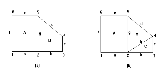
In ArcInfo, locational information about geographic features is represented by three classes of spatial objects: points, arcs, and polygons. Descriptive information about the geographic features is considered the attributes of spatial objects and is stored in relations of relational databases. To extend ArcInfo by giving temporality to both spatial and attribute information, all spatial objects and attributes are time-stamped. The versioning technique we chose is at the record or tuple level. Figure 1 shows the time stamps for point, line, and polygon attribute tables. These tables may be the common database tables such as those with an extension .DBF in ArcInfo, or arc, point, and polygon attribute tables, which, in ArcInfo have the extensions .ATT (arc attribute tables) and .PAT (point and polygon attribute tables), respectively.
Figure 1. Polygon Coverages in 1994 and 1996
| TAZ_ID | Vd_From | Vd_From | DB_From | DB_To | Area | Perimeter |
|---|---|---|---|---|---|---|
| A | 19940101 | 9991231 | 19940131 | 99991231 | 14.00 | 15.00 |
| B | 19940101 | 19951231 | 19940131 | 19951214 | 8.24 | 12.20 |
| B | 19960101 | 99991231 | 19951215 | 99991231 | 5.53 | 10.90 |
| C | 19960101 | 99991231 | 19951215 | 99991231 | 2.71 | 8.10 |
| Arc_ID | Vd_From | Vd_From | DB_From | DB_To | F_Node | T_Node | L_Poly | R_Poly |
|---|---|---|---|---|---|---|---|---|
| a | 19940101 | 99991231 | 19940131 | 99991231 | 1 | 2 | A | 0 |
| b | 19960101 | 99991231 | 19951215 | 99991231 | 2 | 3 | C | 0 |
| b | 19940101 | 19951231 | 19940131 | 19951214 | 2 | 3 | B | 0 |
| c | 19960101 | 99991231 | 19951215 | 99991231 | 3 | 4 | C | 0 |
| c | 19940101 | 19951231 | 19940131 | 19951214 | 3 | 4 | B | 0 |
| d | 19940101 | 99991231 | 19940131 | 99991231 | 4 | 5 | B | 0 |
| e | 19940101 | 99991231 | 19940131 | 99991231 | 5 | 6 | A | 0 |
| f | 19940101 | 99991231 | 19940131 | 99991231 | 6 | 1 | A | 0 |
| g | 19940101 | 99991231 | 19940131 | 99991231 | 2 | 5 | A | B |
| h | 19960101 | 99991231 | 19951215 | 99991231 | 2 | 4 | B | C |
| TAZ_ID | Vd_From | Vd_From | DB_From | DB_To | Population | Employment |
|---|---|---|---|---|---|---|
| A | 19900401 | 99991231 | 19901031 | 99991231 | 66,682 | 14,000 |
| B | 19900401 | 99991231 | 19901031 | 19951214 | 47,089 | 4950 |
| B | 19900401 | 99991231 | 19951215 | 99991231 | 31,602 | 3322 |
| C | 19900401 | 99991231 | 19951215 | 99991231 | 15,486 | 1628 |
The geographic area in the examples is a transit corridor along Southwest 40th Street in Miami. The bus route has undergone many changes. Using the temporal GIS query, changes in both the bus route alignment and the characteristics of the service area along the bus route may be examined. In Figure 2, changes in bus Route 40 between June 15, 1986, and December 31, 1990, are shown. The map is generated by applying the PERDCOV command, which retrieves all the arc segments of the bus route and all the point features representing the bus stops that are effective (or valid) in the given time period. The bus route alignment database is created using the present MDTA bus route GIS map, with older alignment segments added based on the route maps published previously. All the arcs are time-stamped.
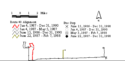
Figure 2. Changes in Bus Route 40 between June 15, 1986, and December 31,
1990
To examine the changes in the factors influencing transit ridership, buffer zones of one quarter
mile (402 meters) are created around the bus stops along Route 40 alignments of 1986 and 1990,
respectively. The buffer zones are then overlaid with the 1986 and 1990 TAZ layers, respectively,
which are produced using SNAPCOV and SNAPINFO and contains the statistics of population,
employment, and school enrollment.
In Figure 3, changes in the population density and employment density in the service coverage area of Route 40 are given in both actual numbers. The numbers are given next to the bus stops for which the data has been generated. When bus stops are closely spaced, their buffer zones overlap, and it is difficult to uniquely allocate population and employment to individual bus stops within the cluster. The connected buffer zones are not separated and the data are given for the entire cluster, which appear in or outside the circles in Figure 3.
From Figure 3, it may be observed that, at some locations, there have been significant changes in population and employment. In the majority cases, the decrease in population is accompanied by an increase in employment, which has been caused by heavy commercial developments such as new shopping centers and strip malls along the bus route. In fact, the total population and employment in the corridor have increased by 45.52 percent and 43.94 percent, respectively. In contrast, bus ridership has increased only slightly between 1987 and 1990. To understand the relationship between ridership and land use and demographics, more detailed study is needed to consider many socio-economic and demographic factors. The detailed ridership data collected by traffic checkers that allow the determination of actual transit usage at bus stops are also needed.
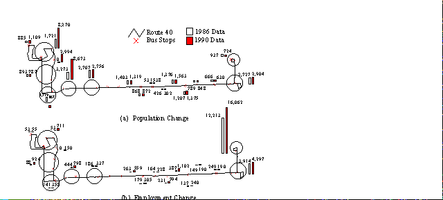
Figure 3. Changes in Population, Employment, and School Enrollment in Route 40 Service
Area between June 15, 1986 and December 30, 1989
Successful temporal GIS applications also rely on the availability of historical data. At present, because of the lack of technologies and tools to store and utilize temporal information, large volumes of data are collected, often with high costs, used, and then either discarded or archived in a way that future use of the data is almost impossible. This is a tremendous waste of resources. Some transportation agencies have begun to realize the value of historical information, but are limited in their ability to utilize the data. With further research on temporal GIS, awareness of the benefits of temporal GIS will be improved. As a result, it is hoped that data collection practices will be improved. In addition, the issues related to the development GIS standards to accommodate temporal information must also be addressed.
Langran, G. (1993). Manipulation and Analysis of Temporal Geographic Information. Proc. of Canadian Conference on GIS, Ottawa, Canada, pp. 869-879.
Peuquet, D. and Wentz, E. (1994). An Approach for Time-Based Analysis of Spatiotemporal Data. Proc. of 6th International Symposium on Spatial Data Handling, Edinburgh, UK, pp. 489-504.
Peuquet, D. and Wentz, E. (1995). An Event-Based Spatiotemporal Data Model (ESTDM) for Temporal Analysis of Geographic Data. International Journal of Geographic Information Systems, Vol. 9, pp. 7-24.
Langran, G. and Chrisman, N. (1988). A Framework for Temporal Geographic Information. Cartographica, Vol. 15, pp. 1-14.
Hazelton, N.W.J., Leahy, F.J., and Williamson, I.P. (1990). On the Design of Temporal Referenced 3-D Geographic Information Systems: Development of Four-Dimensional GIS. Proc. of GIS/LIS '90, Anaheim, CA, pp. 357-372.
Peuquet, D. (1994). It's About Time: A Conceptual Framework for the Representation of Temporal Dynamics in GIS. Annals of the Association of American Geographers, Vol. 84, pp. 441-461.
Kelmelis, J. (1991). Time and Space in Geographic Information: Toward a Fourth-Dimensional Spatio-Temporal Data Model, Ph.D. dissertation, Dept. of Geography, Pennsylvania State University.