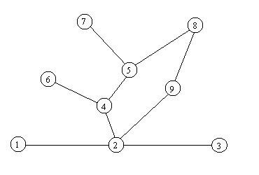
Figure 1: Pictorial Representation of a Graph
The presentation focuses on the algorithm and how it complements the analysis available using only the facilities embedded in a typical commercial GIS, such as Esri's ArcInfo. Examples are included that show how the algorithm computes and records arc restriction attributes, how it can be utilized to display which portions of the road network are restricted for a given set of dates, and how it complements other types of analyses that determine road density by date, total accessible road distance by date, and nonaccessible or roadless areas.
This is the motivation for the problem investigated here: finding a way to identify which portions of a road network are restricted by a set of barriers, and in addition, determining the nature of the restrictions imposed by the barriers. This also includes answering questions such as when are the road segments restricted, to which vehicle types are the restrictions applied? A road may be closed by placing a gate on the road or by a more permanent means such as a kelly hump or revegetation. If any road leading into a subset of the network has not been closed, access to the subnetwork has not been adequately restricted.
The determination of which road segments are restricted is dependent on the restrictions imposed by the barriers. When determining whether access past a barrier is possible, the answer may not be "YES" or "NO" but the answer might also be "MAYBE". That is, it is necessary to not just identify where the barrier is located, but also when the barrier is closed and to which vehicle classes it is closed. For example, two gates may be placed on a road, intending to close the road between the gates. If the first gate is permanently closed and the second gate is only closed seasonally, the restricted portion of the road between the gates is only closed seasonally, regardless of the fact that the first gate is permanently closed. An additional aspect of the seasonal nature of gates occurs when gates with different closure dates close the same subnetwork of the road network. When the closure dates of the gates do not coincide, the effective closure period of the affected road subnetwork is the intersection of the closure periods of the associated gates. Gates may also impose different restrictions on different classes of vehicles. A gate may specify that automobiles may not proceed past the gate at any time while all terrain vehicles (ATVs) may go past the gate for a portion of the year (say May 1 through October 15) and snowmobiles may proceed past the gate during a different part of the year (say December 1 through March 30.)
Many organizations which are responsible for natural resource management rely on data which indicates when road segments are accessible and when they are not. This data assists in critical decision support issues concerning the area impacted or serviced by the road network. Even though road network information is becoming available in digital form, the analysis is still most often done manually. One manager who is responsible for finding these restriction attributes reports that the effort to perform the analysis manually generally takes many person-months of effort. Other factors make a manual analysis less than desirable besides the labor cost. Many organizations manage road systems which resemble a plate of spaghetti. When attempting to determine the restrictions imposed on a particular road segment, it is hard to assure that the person manually performing the analysis has identified every possible path which affects the accessibility of that road segment. Another factor which makes manual attribution undesirable is the fact that few road systems are static. Barriers are routinely added or removed, barrier closure schedules are changed, and roads are built or abandoned. In a complex network, barrier and road changes can have dramatic and widespread effects. Generally a complete analysis should be performed prior to any change to predict the potential effects, and again following any change to record the effects. Maintaining a complete and consistent analysis is thus much harder and more error prone than simply attributing the road network once when digital information first becomes available.
Ideally, an automated analysis tool would be used to perform the analysis, allowing the restricted road segments to be identified and attributed in a matter of minutes. Besides requiring significantly lower labor cost to perform the analysis, this reduces the impact of human errors. An automated tool would also allow the managing organization to run simulations to determine the effects that barrier and/or road changes can have on the road network. Without the availability of a tool of this nature, it might not be possible or cost effective to a priori determine the effects of large sets of additional gates.
In addition to labor cost savings, the data generated by this effort can be utilized as input by many additional types of analysis. For example, many types of analysis involve determining road closure alternatives that ensure that access into an area has been restricted. The restricted area can range from a sensitive wildlife habitat to a recreation area that has suffered ill-effects from excessive human use. This analysis can focus on finding a simple solution, an "optimal" solution or a set of solutions for public comment. A simple solution involves determining the placement of a set of gates (or other closure mechanisms) that ensure that every path into the area is closed. It does not attempt to quantify or optimize the placement of these gates in any way, but just makes sure all routes into the area are closed. An optimal solution tries to accomplish area closure and meet some sort of quantitative criteria. For example, an optional solution might elect to close a set of gates to minimize the number of new gates that need to be installed, minimize the distance gates are from a main road, or minimize the area outside the closed area that is affected by the road closures. A set of possible solutions might try to find all solutions that satisfy some specified cost constraints. Other similar types of analysis involve identifying nonaccessible or roadless areas which lie within the region serviced or impacted by the road network, or within a given distance of an accessible road segment on the network.
Other analyses can utilize data generated by this effort as input. These analyses include but are not limited to the following topics: identifying which parts of a road system are closed to traffic when a specific gate at a specific point of a road network is closed or open; determining an area's resulting road density (distance of accessible roads in the polygon divided by the size of the area) when a portion of the road subnetwork in the area is closed; determining the effect on travel distance between points when gates are opened or closed; and finding good or optimal routes that allow staff to manually close a set of gates.
Figure 1: Pictorial Representation of a Graph
We can assume that a simple graph can be represented with a GIS line coverage, which records lists of nodes and arcs. Both nodes and arcs can be attributed by having special information attached to them; we assume that such information is stored in either a Node Attribute Table or Arc Attribute Table, that provide attribute information about a graph. Generally this information is used to help identify to which class a particular node or arc belongs, and to record other data specific to nodes and arcs. For example, to reflect the times when vehicle traffic access is restricted on parts of the coverage, we assumed that all nodes and arcs have a not-accessible-dates (NAD) attribute. This attribute defines the set of days when different vehicle classes are known to be restricted from accessing the road network at that location. Initially, this attribute has the value "undefined" for each member of the graph.
The objective of the road analysis problem from a graph theory perspective is to represent a road network with a particular type of graph, assign initial attribute values to some nodes, then compute other key attribute values for other member arcs and nodes. Any type of graph analysis is sensitive to the size of the graph. The road closure analysis only needs to consider the portion of the road network which is local to the analysis area. For example, if road closures are being analyzed in the Bitterroot National Forest, it is not necessary to include all the roads in the United States in the graph. Including more of the road network than necessary in the graph will hamper performance of the analysis. Intuitively, including the roads that lie within or near the analysis area in the analysis graph will suffice, but it may be difficult to determine just which roads to include or exclude before doing the analysis.
In some instances the size of the graph needed to include the surrounding loop of highways can be quite large. It may not be feasible to expect the organization doing the analysis on the study area to translate the whole road network into a graph so as to achieve this goal, especially if a large portion of the road network lies outside their jurisdiction. As a result, the main road or highway may or may not be included in the graph. In the event that the main road or highway is not included in the graph, special nodes of degree equal to one, called access nodes, are introduced to summarize the accessibility. The arc from such a point leads into the road network of interest; as explained below, data attributes at this point abstract the access to/from the outside world. Typically, access points are identified when the graph is first reduced from a larger network.
As an interface between the study graph and the outside world, each access point has an initial-not-accessible-dates (INAD) attribute, which lists the set of days when different vehicle classes are known to be restricted from accessing the road network from the outside at that location. For example, if an access point can only be reached by passing through a gate which is closed January 1 through May 15, the access point's INAD has the value {Jan 1, Jan2, ... , May 15}. If the access point can be reached at any time in the year its INAD is empty. If there are multiple paths off the graph from the highway to the access point, its INAD will be the intersection of the restrictions on accessibility for each of the paths. For example, if one path to an access point to a highway is closed January 1 through June 15 and another path is closed April 1 through July 31, the access point's INAD is {Apr 1, ... , June 15} If a single path to an access point includes more than one barrier, the dates vehicle traffic can obtain access along that path is the intersection of the dates each barrier along that path restricts traffic.
Another class of nodes which is of interest in road closure analysis are barrier nodes, which record activities on the road network which have the ability to restrict traffic flow. Examples of barriers include gates, washouts, kelly humps, revegitation, and travel management signs. In graph terms, a barrier is represented as a node with degree equal to two with a barred-access-dates (BAD) attribute which lists the set of dates the barrier restricts traffic flow.
In review, there are four steps that must be taken to represent a road network as a graph. The steps are as follows.
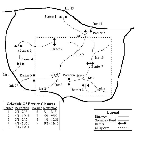
Figure 2: A Simple Road Network
As an example, consider the simple road network illustrated in Figure 2, which shows both highways, secondary roads, and barriers. The study area is represented as a dashed rectangle. A schedule of barrier closures specifies when each of the barriers is closed. The graph representation of the same road network, restricted to the study area, is illustrated in Figure 3. The graph contains three classes of nodes. Nodes with a label A represent access point nodes, nodes with a label B represent barrier nodes, and nodes which are only labeled numerically represent intersection points in the road network, i.e., nodes that are neither access points or barriers.
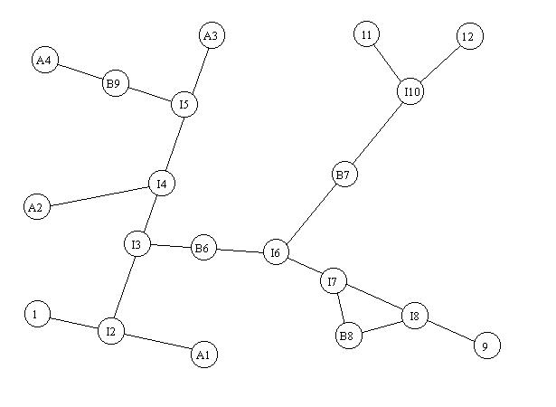
Figure 3: Graph Representation of a Road Network and Study Area
Figure 4 shows a table of INAD and BAD values for access point and barrier nodes. For example, access point A3 corresponds to the point where the path from the highway which passes through Barrier 1 and the path from the highway which passes through Barrier 2 enter the study area. Barrier 1 is closed February 1 through July 15 and Barrier 2 is closed April 1 through October 15. A3's resulting INAD attribute is {April 1, ... July 15} which is the intersection of the INADs for the paths to the access point, i.e., {2/1..7/15} intersect {4/1..10/15} = {4/1..7/15}. Barrier node B6 has a BAD attribute value of {3/1..7/15} which is derived from Barrier 6's entry in the schedule of closures. Figure 4 lists the INAD and BAD attribute values for the barrier and access point nodes of the graph shown in Figure 3.
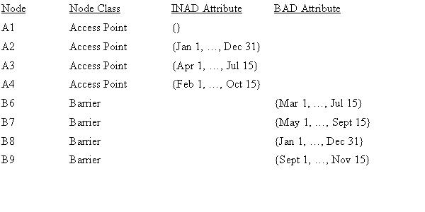
Figure 4: Barrier and Access Point INAD and BAD Attribute Values
Given a graph with access point and barrier information, the goal is to determine the affects of the barrier and access point INAD attributes on the NAD attributes of the graph's member arcs. To do this, we note that a connected element set (CES) is a set of nodes and arcs which can be reached from X without passing through any barrier. These sets include arcs that are associated with a barrier, but do not include any barrier nodes. It is assumed that each connected element set has a not-accessible-dates (NAD) attribute, which has the same value as the NAD attribute of all members of that connected element set. Each set also has an INAD attribute, which is computed as the intersection of the INAD attributes for each of the set's member access points. If none of the member nodes are access points, the set's INAD attribute value is unknown. The graph shown in Figure 3 has four connected element sets. The table in Figure 5 shows their members and INAD attributes.
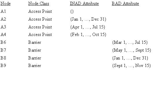
Figure 5: Connected Element Sets
Note that the arcs on either side of barrier node B8 are in the same connected element set
(CES3). This is a result of the path which exists between the arcs associated with B8 (i.e.
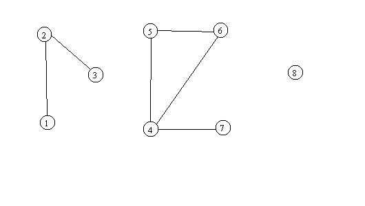
Figure 6: Connected Graph Components
The basic connected-components algorithm takes a standard graph as input. Each node on the graph is initially put into a connected component set by itself. The algorithm examines each arc in the graph. As each arc is processed, each node to which it is connected via an arc is identified. If both source and target nodes are contained in different connected component sets, the two sets are merged. If both nodes are already in the same connected component set, no further action is required for that arc. When the algorithm completes, each node in any connected component set may be reached from any other node in the same connected component set by following a path of arcs in the graph.
The basic connected-components algorithm does not explicitly indicate which arcs connect the nodes in a connected component set, and must be extended to handle barriers, especially ones that are closed seasonally. As mentioned previously, a node representing the barrier is attributed to indicate when traffic access is restricted. The classic algorithm assumes that each node will end up in one and only one connected component set, and does not check the attributes on barrier nodes to adjust connectivity. Although a barrier is reachable from the two connected component sets on either side of the barrier, the barrier is not a member of either connected set.
The derivative algorithm CONDITIONAL-CONNECTED-COMPONENTS (CCC), shown in Figure 7, keeps the node representing the barrier in a connected set by itself. This connected set is labeled as a barrier and is attributed with any restrictions the barrier imposes on traffic access. It is also linked via barrier links to the connected sets containing the nodes on either sides of the barrier. These barrier links allow the derivative algorithm to identify the impact of the barrier's restrictions on access from the neighboring connected sets. CCC also utilizes a construct to group connected graph members (both arcs and nodes) in a special structure referred to as a connected set. In order to attribute arcs with the access restrictions identified for the associated nodes it is necessary to associate the set of connected nodes and the arcs in the same data structure. A connected set originates in the same way as a connected component set, with each node in the graph being placed in a connected set by itself.
CCC processes arcs one by one. If both nodes are in the same connected set, the arc is placed in that connected set. If neither node is a barrier and the two nodes are in different connected sets, the connected sets are merged and the arc is placed in the merged connected set. If neither node is a barrier, the arc joining them is put in the connected set with its end points. If one of the nodes represents a barrier, the arc is placed in the connected set which contains the arc's nonbarrier node and a barrier link is also established between the two connected sets. If both nodes associated with an arc are barriers, a pseudo connected set is created which contains no nodes, but has the arc and links to the connected sets containing the two nodes.
The CCC algorithm requires a slightly different data structure than the classic connected-components algorithm. CCC uses a data structure of sets, where each set consists of a list of connected nodes and a list of associated arcs. Each connected set contains a list of references to the connected sets containing neighboring barrier nodes. Connected sets contain a INAD and NAD attributes. Calculation of values for these two attributes is addressed in the following section. CCC's data structures must support the following operations.
As shown in Figure 7, the procedure CONDITIONAL-CONNECTED-COMPONENTS uses the preceding disjoint set operations to group together connected graph components with barriers. Once CCC produces its results, it is possible to determine whether two nodes are on the same connected set by comparing the results of running FIND-SET for both nodes. If the same connected set is returned by both calls, then the nodes reside on the same connected set; otherwise they are in different connected sets. The set of nodes from graph G is denoted N[G], and the set of arcs is denoted by A[G]. In solving the road closure analysis problem, once the procedure CCC produces its results, the NAD attributes for each connected set can be determined, as discussed below. The NAD attribute for each set can be recorded with each of its member arcs once the attribute is determined for the connected set.

Figure 7: CONDITIONAL-CONNECTED-COMPONENTS Algorithm
NAD attribute determination is performed using an iterative breadth first search. The NAD attributes that are calculated for any connected set apply to each of its member arcs and nodes. The first step in calculating NAD values is to identify the connected sets which have known INAD values, based on the member access points they contain which have an INAD attribute. This is determined for each connected set by taking the intersection of each member access point's INAD attribute.
Next an iterative breadth first search is done of the collection of connected sets. Each breadth first search starts by placing each connected set which is known to have unlimited access onto a queue and setting its NAD attribute to the empty set. As each set on the queue is processed, all neighboring sets which have not been previously placed on the queue in the current search iteration are pushed onto the queue. As each set is pulled off the queue, it's NAD attribute is updated by taking the intersection of it's current NAD (if known), its INAD (if it has one) and the effective restrictions imposed by each neighboring barrier. The effective restriction imposed by a neighboring barrier can be determined only if the NAD of the connected set on the other side of the barrier is known. If that NAD is known, the effective restriction of the barrier is union of the barrier node's BAD attribute and the NAD attribute of the connected set lying on the other side of that barrier from the connected set currently being processed. This breadth first search is repeated until the NAD attribute for each connected set are the same as they were after the previous breadth first search.
The first phase of the analysis involves access point management. Access points are locations on the road network that are known to be accessible to vehicle traffic. It is possible for there to be restrictions on when certain vehicles may have access at the specified location. These points may correspond to highways or other roads which are designated as being open to vehicles.
The analysis tool provides a way for the user to add access points to a point coverage and specify accessibility attributes to be associated with the access points. The accessibility attributes specify when vehicle traffic is known to be able to have access to the road network at the access points. The portion of the toolset which is used for this part of the analysis is implemented as an Arc Macro Language (AML) script. The script utilizes ArcInfo's ArcEdit module to add user specified access points to a point coverage which stores access points. ArcEdit displays the road coverage, allows the user to graphically specify the location of access points to be stored in the corresponding point coverage with the ADD command, and attributes the access point with its accessibility attribute via the MOVEITEM command.
The Forest Service does not have a rule system or data set which specifies information about access points, nor do any of their GIS databases have these access points recorded. It is assumed that vehicles can always gain access to any location on a highway, other main road, or a node on the edge of the coverage which is known to be accessible to a highway by a road which is not on the road coverage.
The second phase of the analysis involves barrier management. Barriers are entered in a manner similar to how access points are added. The analysis tool provides a mechanism allowing the user to add barriers to a barrier point coverage and allows for associating restriction attributes with the barriers. The portion of the toolset which is used for this part of the analysis utilizes an AML script which is similar to the script used for the management of access points. The script utilizes ArcInfo's ArcEdit module to add user specified barriers to a point coverage which stores the user specified barriers. ArcEdit displays the road coverage, allows the user to specify the location of barriers to be stored in the corresponding point coverage with the ADD command, and attributes the barriers with the nature of the restriction imposed on traffic flow by the barrier with the MOVEITEM command.
Another option for storing barrier data which was not utilized in this project is to utilize an Oracle database system called the Route Management System (RMS). Each entry in the RMS specifies with which road a barrier is associated, in addition to where on that road the barrier is located. By using ArcInfo's dynamic segmentation, we could model linear features using routes and events. A route represents a non-circular series of connected arcs, along with measures which can be used to calculate distance. Events are locations of interest along a route (e.g. barriers, bridges, signs, etc.). Distance measures can also be used to identify the location of events along a route (Esri, 1995B). Dynamic segmentation is a process based on events and routes which allows arcs which contain specified events (e.g. barriers) to be identified along with where on the route (i.e. which arc) the event is located. Using dynamic segmentation, barriers in the RMS can be co-registered onto the associated road network as nodes.
Although dynamic segmentation could have definite applicability to road closure analysis in the future, its use needs to be augmented with point representation of barriers to produce an analysis tool capable of allowing users to determine the effects of new barriers or modified closure schedules on existing barriers. Currently, no forests have an RMS mature enough to reliably represent the existing set of barriers, and the RMS that are available are not generally accessible outside the Forest Service.
The CONDITIONALLY-CONNECTED-COMPONENTS analysis program is run on the road coverage, which now includes the barriers and access points represented as attributed nodes. The CCC program accesses the road coverage by reading ASCII copies of the road coverage's AAT and NAT, which have been dumped as ASCII files from ArcInfo via the UNLOAD command. The analysis program produces an Arc Restriction File as an ASCII output file, which records the arcs found to have restrictions and the nature of those restrictions. This file can be loaded into a newly created ART via the ArcInfo ADD command.
The CONDITIONALLY-CONNECTED-COMPONENTS analysis program can achieve additional performance by modifying the implementation to directly access tables within ArcInfo, rather than exporting and importing ASCII files. The tables can be directly accessed by using facilities in either Arc Software Developers Library (ArcSDL) or Infolib. ArcSDL is a C application programming interface developed by Esri which allows C/C++ applications to directly access ArcInfo data structures and invoke ArcInfo commands from within an application. While a copy of ArcSDL is available in the University of Montana Computer Science Department, it is not used in this effort because distribution and support for ArcSDL is highly restricted. Another means of directly accessing the ArcInfo tables is using Infolib. Infolib is an unsupported C library which allows applications written in C/C++ to directly access the ArcInfo tables. Infolib was developed by Esri and is available free at many sites on the Internet. However, Esri makes it clear that this library is not officially supported, so its use in any long term project is also questionable. This, any development of a more robust means to interface the CCC program and ArcInfo is dependent on Esri's ability and willingness to provide standard interface libraries to their data formats.
The last phase of the analysis entails utilizing the analysis tool's visualization script to view what impact the barriers have on the road network. This crude visualization mechanism is implemented as an AML script. The script allows the user to specify visualization criteria including begin date, end date and vehicle class. The script calls a C++ program which examines the ART to identify which arcs are restricted from the specified begin date through the specified end date for one or more of the vehicle classes specified. The script then utilizes ArcInfo's ArcPlot module to graphically display the road network. The color used to display an arc signifies how many of the specified vehicle classes are restricted for that arc. Which colors are used is dependent on the local symbol file being used by ArcInfo. When using the default symbol table, white signifies arcs that are not restricted for any specified vehicle class, red arcs are restricted for specified vehicle class one, green for vehicle class two, and blue for vehicle class three. The script also identifies arcs which are found to not be on any path to any access point. This visualization script may be run multiple times for different sets of dates and vehicle classes.
[Cormen90] T.Cormen, C.Leiserson, R.Rivest, Introduction to Algorithms. MIT Press, Cambridge, Massachusetts, 1990.
[Hamilton97] D.Hamilton, Analysis of Road Network Accessibility. M.S. Thesis, Department of Computer Science, University of Montana, May 1997.