Michael J. Gilbrook
ABSTRACT
HDR Engineering used a combination of GIS tools to locate a feasible road corridor through the southern Appalachian Mountains of north Georgia for the Georgia Department of Transportation. An ArcInfo least-cost path model employing twenty-eight GRID layers identified potential routes in Phase I. Throughout all three Phases, ArcInfo quantified potential environmental impacts and engineering considerations for potential corridors such as historic sites, wetlands, stream crossings, historical accident data, and vertical profiles. We employed ArcView GIS to explain the study's findings to residents at public meetings using the same GIS coverages that drove the analysis.
INTRODUCTION
The Appalachian Scenic Corridor Study (ASCS) was a two-year project conducted under contract by HDR Engineering, Inc. for the Georgia Department of Transportation (GDOT) Office of Planning. The purpose of the study was to evaluate the need for, and feasibility of, a continuous east-west transportation link across north Georgia from I-85 in Franklin County to I-59 in Dade County. The recommended corridor had to serve economic development of North Georgia and accommodate future traffic demand, while blending into the environmental and cultural milieu that makes the southern Appalachians such an attractive place to live.
From its inception, the ASCS was conceived as a project which would rely on GIS as the centerpiece for all project related activities, including:
This paper outlines how the Esri family of GIS software products was used to address each of these activities.
PHASE I: INITIAL CORRIDOR IDENTIFICATION PROCESS
Ideally, a transportation corridor between any two points should take the shortest route possible which also minimizes adverse impacts to natural resources, cultural features, and human populations. The best routes should also avoid areas of difficult terrain, crossings of large bodies of water, and other adverse physical features. Finally, the ideal route should follow those areas of existing road which are suitable for inclusion in the transportation corridor. Evaluating all these constraints simultaneously is difficult for human beings, but much easier for a computer. Phase I of the ASCS project used the ArcInfo GRID modeling technique called Least-Cost Path Analysis to help the Project Team identify potential transportation corridors. The methodology included the following steps:
Developing Least-Cost Path Ranking Criteria
In order to generate a "cost-surface" or combined constraints map, individual maps representing each of the input criteria of interest were individually ranked on a common scale. The ranking criteria developed for each data theme were based on a scale of 1 to 5. Such a scale provided sufficient refinement for capturing shades of difference in any given data theme, yet kept the number of categories to a number which could be easily interpreted and understood. The five levels could be thought of like this:
|
TABLE 1 Interpretation of Constraints Map Ranking |
||
|
Ranking |
Constraints For Corridor |
Suitability For Corridor |
|
1 |
Very Low |
Very High |
|
2 |
Low |
High |
|
3 |
Medium |
Medium |
|
4 |
High |
Low |
|
5 |
Very High |
Very Low |
The table illustrates that any data layer could be thought of in terms of either constraints or suitability. Constraints were those things that, when present, would be bad for transportation corridor development. The lower the constraints score, the fewer the obstacles to development. Suitability was the converse; areas with a low rank (i.e., 1 or 2) had conditions that were very suitable for transportation corridor development. The terms suitability and constraints are largely interchangeable, as long as one realizes that the rankings run from very low to very high for constraints, but from very high to very low for suitability. Table 2 lists the input themes to the least-cost path model, and shows how attributes in each theme were ranked in terms of transportation corridor constraints and/or suitability.
|
TABLE 2 Ranking Of Input GRIDs for Phase I Least-Cost Path Analysis |
||||||
|
Data Theme |
Very Low (Rank 1) |
Low (Rank 2) |
Medium (Rank 3) |
High (Rank 4) |
Very High (Rank 5) |
Source |
|
Archeological Site Potential |
Areas Of Limited Archeological Potential |
N/A |
N/A |
N/A |
Areas Of High Archeological Potential |
New South |
|
Bicycle Route Designation (Roadway) |
Not Designated As Bicycle Route |
N/A |
N/A |
N/A |
Designated As Bicycle Route |
GDOT, RDC, County Plans |
|
Bicycle Route Designation (Parkway) |
Designated As Bicycle Route |
N/A |
N/A |
N/A |
Not Designated As Bicycle Route |
GDOT, RDC, County Plans |
|
Historic Districts * (Roadway) |
> 0.5 mi From Historic Districts |
N/A |
N/A |
N/A |
< 0.5 mi From Historic Districts |
Jaeger Co., Various |
|
Historic Districts * (Parkway) |
> 0.25 mi From Historic District |
N/A |
N/A |
< 0.25 mi From Historic District |
Historic District |
Jaeger Co., Various |
|
Historic Sites * (Roadway) |
> 0.5 mi From Historic Sites |
N/A |
N/A |
N/A |
< 0.5 mi From Historic Sites |
Jaeger Co., Various |
|
Historic Sites * (Parkway) |
> 0.25 mi From Historic Site |
N/A |
N/A |
< 0.25 mi From Historic Site |
Historic Site |
Jaeger Co., Various |
|
Scenic Roadway Corridors (Roadway) |
Non-Designated Roadways |
N/A |
N/A |
N/A |
Designated Scenic Roadway Corridors |
GDOT, Various |
|
Scenic Roadway Corridors (Parkway) |
Designated Scenic Roadway Corridors |
N/A |
N/A |
N/A |
Non-Designated Roadways |
GDOT, Various |
|
Conservation Areas** (Roadway) |
> 3 mi, < 10 mi From Recreational Area |
N/A |
N/A |
< 3 mi , > 10 mi From Recreational Area |
Recreational Area |
SAA, Various |
|
Conservation Areas ** (Parkway) |
> 1 mi, < 5 mi From Recreational Area |
> 5 mi, < 10 mi From Recreational Area |
N/A |
< 1 mi , > 10 mi From Recreational Area |
Recreational Area |
SAA, Various |
|
USFS Wilderness Areas ** (Roadway) |
> 10 mi From Wilderness Area |
N/A |
N/A |
< 10 mi From Wilderness Area |
Wilderness Area |
SAA, Various |
|
USFS Wilderness Areas ** (Parkway) |
> 5 mi From Wilderness Area |
N/A |
N/A |
< 5 mi From Wilderness Area |
Wilderness Area |
SAA, Various |
|
Existing Mine & Quarry Locations |
> 0.5 mi From Mines or Quarries |
N/A |
N/A |
N/A |
0.5 mi Around Mines or Quarries |
USGS, GDNR |
|
Existing Non-Road Corridors (Roadway) |
Rail, Utilities or Transmission Lines |
N/A |
N/A |
N/A |
No Corridors |
GDOT Roadways |
|
Existing Non-Road (Rail, Utilities or Transmission Lines) Corridors (Parkway) |
Rail & Utility Corridors |
N/A |
N/A |
N/A |
No Corridors, Transmission Lines |
GDOT Roadways |
|
Existing Roadway Right-Of-Way Width |
> 200' |
150' - 200' |
100' - 150' |
< 100' |
All Other Roads |
GDOT Roadways |
|
Roadway Access Control |
Fully Controlled Access |
N/A |
Partially Controlled Access |
N/A |
Uncontrolled Access |
GDOT Roadways |
|
0m - 300m |
N/A |
300m - 500m |
N/A |
> 500m |
USGS DEM |
|
|
Surface Slopes |
0 - 15 deg |
N/A |
16 - 25 deg |
N/A |
>= 26 deg |
USGS DEM |
|
Truck Route Designation (Roadway) |
Designated Truck Routes |
N/A |
N/A |
N/A |
Not Designated As Truck Route |
GDOT Roadways |
|
Truck Route Designation (Parkway) |
Not Designated As Truck Route |
N/A |
N/A |
N/A |
Any Truck Route Designation |
GDOT Roadways |
|
0 mi - 2 mi From Boundary Of High Intensity Urban |
N/A |
> 2 mi From Boundary Of High Intensity Urban |
Low Intensity Urban |
High Intensity Urban |
SAA |
|
|
Very Low |
Low |
Medium |
High |
Very High |
SAA |
|
|
Game Species Habitat Potential |
0 species |
6 species |
8 species |
9 species |
10 species |
SAA |
|
Land Cover |
Bare Soil, Herbaceous, Pasture, Urban |
Crops |
Forests |
Wetland, Rock Outcrops |
Water |
SAA |
|
TNC Listed Species Habitat Potential |
No Listed Species Habitat |
1 - 4 species |
5 - 47 species |
49 - 69 species |
>= 70 species |
SAA, TNC |
|
USFWS Listed Species Habitat Potential |
No Listed Species Habitat |
1 species |
8 - 10 species |
11 species |
12 - 15species |
SAA, TNC |
|
Keystone Species Habitat Potential |
0 species |
N/A |
2 species |
3 species |
4 species |
SAA |
|
High Management Species Habitat Potential |
0 species |
<= 4 species |
4 - 15 species |
16 - 19 species |
> 19 species |
SAA |
|
Population Density |
Very Low Population Density |
Low Population Density |
Medium Population Density |
High Population Density |
Very High Population Density |
US Census TIGER |
|
Existing Roadway Speeds |
Speed Limit > 55 mph |
Speed Limit > 45, < 55 |
Speed Limit > 35, < 45 |
Speed Limit > 25, < 35 |
Speed Limit < 25 |
GDOT Roadways |
|
Existing Traffic Volumes |
Any Road, > 10K ADT |
Rural Roads, 5K - 10 K ADT |
Rural Roads, < 5K ADT |
Urban Roads, 5K - 10 K ADT |
Urban Roads, < 5K ADT |
GDOT Roadways |
|
Number Of Lanes (Roadway) |
>= 4 Lanes |
N/A |
3 Lanes |
N/A |
2 Lanes |
GDOT Roadways |
|
Number Of Lanes (Parkway) |
2 Lanes |
3 Lanes |
N/A |
N/A |
>= 4 Lanes |
GDOT Roadways |
|
Road Traffic Congestion |
V/C < 0.6 |
V/C > 0.6, V/C < 0.7 |
V/C > 0.7, V/C < 0.8 |
V/C > 0.8, V/C < 0.9 |
V/C > 0.9 |
GDOT Roadways |
|
East-West Roads |
N/A |
N/A |
North-South Roads |
Non-Road Areas |
GDOT Roadways |
|
|
Truck Usage (Roadway) |
Trucks > 16% |
Trucks >12%, < 16% |
Trucks >8%, < 12% |
Trucks >4%, < 8% |
Trucks < 4% |
GDOT Roadways |
|
Truck Usage (Parkway) |
Trucks < 4% |
Trucks >4%, < 8% |
Trucks >8%, < 12% |
Trucks >12%, < 16% |
Trucks > 16% |
GDOT Roadways |
|
Notes
|
||||||
GRID Overlay Methodology
The Project Team prepared the ranking critieria in Table 2 as if all data themes had equal importance. However, the Team recognized that a different emphasis on the input criteria might favor least-cost paths sensitive to factors in ways that would be important to distinquishing between alternative transportation facility concepts. For example, to get the best, least-cost path for a high-speed road optimized for transport of goods the following data themes should be considered more important than others: existing roadway suitability, topography, economic development potential. To get the best paths for a scenic parkway concept, we might want to give higher weight to viewshed potential, proximity to parks and low population density areas.
To evaluate the effect of alternative weighting schemes, six cost-surface coverages were generated, each representing the results of different weighting schemes applied to the input coverages. The weighting scenarios were identified as follows:
The Baseline model represented the average of all input layers, each treated as if it had the same importance or weight. The other models varied the weights on the input layers so as to emphasize (or de-emphasize) a given set of constraints or suitability factors which together would suggest transportation corridors sensitive to a certain set of requirements. The weights for each alternative model appear in Table 3.
|
TABLE 3 Alternative Weights For Phase I Least-Cost Path Models |
||||||
|
Input GRID Layer |
Alternative Weighting Scenarios |
|||||
|
Baseline |
Roadway |
Parkway |
Rail |
Environmental |
Engineering |
|
|
Archeological Site Potential |
1 |
1 |
1 |
1 |
2 |
1 |
|
Bicycle Route Designation (Roadway) |
1 |
1 |
N/A |
N/A |
1 |
1 |
|
Bicycle Route Designation (Parkway) |
N/A |
N/A |
2 |
N/A |
N/A |
N/A |
|
Historic Districts * (Roadway) |
1 |
1 |
N/A |
1 |
2 |
1 |
|
Historic Districts * (Parkway) |
N/A |
N/A |
2 |
N/A |
N/A |
N/A |
|
Historic Sites * (Roadway) |
1 |
1 |
N/A |
1 |
2 |
1 |
|
Historic Sites * (Parkway) |
N/A |
N/A |
2 |
N/A |
N/A |
N/A |
|
Scenic Roadway Corridors (Roadway) |
1 |
1 |
N/A |
N/A |
1 |
1 |
|
Scenic Roadway Corridors (Parkway) |
N/A |
N/A |
2 |
N/A |
N/A |
N/A |
|
State Parks & USFS Wildlife Managment Areas ** (Roadway) |
1 |
1 |
N/A |
N/A |
2 |
1 |
|
State Parks & USFS Wildlife Managment Areas ** (Parkway) |
N/A |
N/A |
2 |
N/A |
N/A |
N/A |
|
USFS Wilderness Areas ** (Roadway) |
1 |
1 |
N/A |
N/A |
2 |
1 |
|
USFS Wilderness Areas ** (Parkway) |
N/A |
N/A |
2 |
N/A |
N/A |
N/A |
|
Existing Mine, Quarry & Landfill Locations |
1 |
1 |
1 |
1 |
1 |
2 |
|
Existing Non-Road Corridors (Roadway) |
1 |
2 |
N/A |
2 |
1 |
2 |
|
Existing Non-Road (Rail, Utilities or Transmission Lines) Corridors (Parkway) |
N/A |
N/A |
2 |
N/A |
N/A |
N/A |
|
Existing Roadway Right-Of-Way Width |
1 |
2 |
1 |
2 |
1 |
2 |
|
Roadway Access Control |
1 |
1 |
1 |
1 |
1 |
1 |
|
Surface Elevations |
1 |
2 |
1 |
2 |
2 |
2 |
|
Surface Slopes |
1 |
2 |
1 |
2 |
2 |
2 |
|
Truck Route Designation (Roadway) |
1 |
2 |
N/A |
1 |
1 |
2 |
|
Truck Route Designation (Parkway) |
N/A |
N/A |
2 |
N/A |
N/A |
N/A |
|
Urban Areas |
1 |
2 |
1 |
2 |
1 |
1 |
|
Black Bear Habitat Potential |
1 |
1 |
1 |
1 |
2 |
1 |
|
Game Species Habitat Potential |
1 |
1 |
1 |
1 |
2 |
1 |
|
Land Cover |
1 |
1 |
1 |
1 |
2 |
1 |
|
TNC Listed Species Habitat Potential |
1 |
1 |
1 |
1 |
2 |
1 |
|
USFWS Listed Species Habitat Potential |
1 |
1 |
1 |
1 |
2 |
1 |
|
Keystone Species Habitat Potential |
1 |
1 |
1 |
1 |
2 |
1 |
|
High Management Species Habitat Potential |
1 |
1 |
1 |
1 |
2 |
1 |
|
Population Density |
1 |
2 |
1 |
1 |
1 |
2 |
|
Existing Roadway Speeds |
1 |
2 |
1 |
1 |
1 |
2 |
|
Existing Traffic Volumes |
1 |
2 |
1 |
2 |
1 |
1 |
|
Number Of Lanes (Roadway) |
1 |
2 |
N/A |
1 |
1 |
2 |
|
Number Of Lanes (Parkway) |
N/A |
N/A |
2 |
N/A |
N/A |
N/A |
|
Road Traffic Congestion |
1 |
2 |
1 |
1 |
1 |
1 |
|
Roadway Direction |
1 |
2 |
1 |
1 |
1 |
2 |
|
Truck Usage (Roadway) |
1 |
2 |
N/A |
2 |
1 |
1 |
|
Truck Usage (Parkway) |
N/A |
N/A |
2 |
N/A |
N/A |
N/A |
|
Notes
|
||||||
For the Baseline model,
the cost-surface coverage was generated using the GRID AVERAGE command in ArcInfo. This resulted in a score for each cell calculated by summing the ranks of all input coverages, and dividing by the number of input coverages. Mathematically, the highest score possible was a five, and the lowest a one. For the other models, the process was different. Using GRID algebra, the scores of the input coverage ranks were individually added; ranks were first multiplied by the appropriate weighting factor, where appropriate. The resulting sum was then divided by the sum of the weights assigned to each input coverage, in order to obtain a weighted average. This ensured that the resulting input would remain on a scale of one to five, and make the results of each alternative model largely comparable to one another.Least-Cost Path Analysis
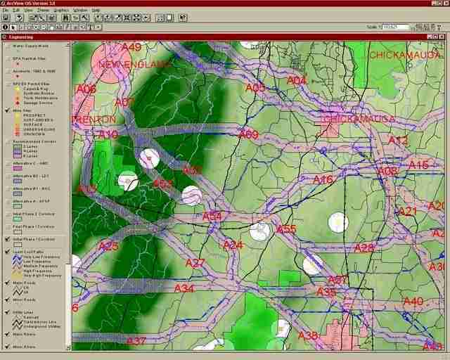
The ArcInfo least-cost path technique allowed the identification of best routes across a given cost surface for many origin points to a single destination. The Project Team identified a series of points which represented the maximum number of logical termini which might conceivably be connected for an east-west trans-Appalachian corridor. These points fell along the break-lines for each of the four study sections into which the project area had been subdivided.
The least-cost path analysis was conducted for the set of all termini on the east side of each section as origin points, leading to each of the termini on the western end as destinations. (The use of the terms "origin" and "destination" here do not having any meaning from a transportation standpoint, but only reflect the direction in which the computer evaluated the least-cost path. The designation of origin and destination could have been switched, and the results would have been the same.) Each least-cost path run for a given terminus was saved as a separate GRID coverage. After all GRID coverages were complete, the least-cost paths were converted to vector lines using the GRIDLINE command. These lines were plotted on 1:100,000 scale maps of each section (along with color-coded maps of the cost-surface coverage) for evaluation by the Project Team.
Corridor Generation & Reduction Process
Following evaluation by the Project Team, a single set of
least-cost path links were combined for each of the four study area sections. These links included nearly all the Baseline model links, plus any of the alternative weighting model links which appeared reasonable based on their superior avoidance of high-constraint areas, or sensitivity to routes with particular high suitability based on one set of values or another. Where multiple paths closely paralleled one another, a single representative path was chosen. Upon further analysis, some termini were deemed unsuitable, and they (and all paths joining them) were deleted. Paths which had extreme north-south orientations, or which otherwise did not exhibit good connectivity with the remaining paths, were also eliminated. Finally, those paths which exhibited some sort of "fatal flaw," such as passing through the center of a conservation area, were also eliminated from further consideration.A series of 0.5 mile corridors for each study area section was prepared by generating a 0.25 mile buffer around the remaining least-cost path centerlines. The buffer coverage was edited to separate the corridors into individual "links," by subdividing the corridor polygons at major intersections. The links were arbitrarily numbered from 1 to n for identification purposes.
The next step in the process required the further reduction of the corridor links. Two GIS methodologies were used to aid the Project Team in evaluating the links. First, the original least-cost paths were combined in GRID to generate a coverage representing the sum of all input coverages. The resulting coverage was used to generate a color-coded plot of paths based on the number of times each path was contributed by an input coverage. Those paths that occurred frequently for multiple pairs of termini and/or from multiple alternative weighting models were deemed high value corridors. This "popularity analysis" was used by the Project Team to evaluate the desirability of functionally equivalent corridors. For example, if two sets of links connected the same set of roadways, then the links exhibiting the greater popularity scores would be preferred.
PHASE II: QUANTIFYING IMPACTS
By the end of Phase I, the Project Team reduced the numerous potential corridors suggested by the least-cost path analysis to less than ten for further study in Phase II. In Phase I, the type of transportation facility (e.g., multi-lane divided highway, or two-lane scenic parkway) did not figure prominently in the corridor evaluation. Minimizing gross environmental and cultural impacts and avoiding engineering difficulties dominated the Phase I evaluation. However, during Phase II the type of transportation facility under consideration had to be factored into the analysis. For the purpose of evaluating Phase II corridors, the Project Team identified three types of routes: (1) Those suitable for "Parkway" concepts, (2) those suitable for "Roadway" concepts, and (3) those suitable for both. Those parts of the Appalachian Scenic Corridor evaluated for the Parkway model would be largely two lanes, with occasional three-lane sections for passing or climbing. The Roadway model presumed a four-lane facility, possibly with a center median. Routes for both models usually followed existing roadways, but would occasionally deviate to form a more direct route for the Roadway alternative.
Throughout all three Phases of the ASCS project, ArcInfo was used to quantify resources within the various corridors being evaluated. These data were generated using the ArcInfo INTERSECT command between coverages containing the corridor alternatives and the resource coverages. For example, the number of acres of potential listed species habitat within each Phase I corridor was calculated by overlaying the corridors on the appropriate coverage. Results were reported by corridor link, which allowed for the impacts of individual links to be compared. This sometimes led to selection of one functionally equivalent link over another as part of the initial corridor identification process. However, most quantitative analysis of corridors occurred during Phases II and III, when the corridors under study had been reduced to a more manageable number and more detailed data were available for each corridor.
Quantification results were often expressed in units of acres per linear mile of corridor, to adjust for the widely varying lengths of the corridor links. Link lengths were obtained by performing an IDENTITY between the corridors (polygon coverages) and the nominal centerlines for those corridors (line coverages). The length of the centerline within a corridor link was taken as the link length. Keep in mind that the "nominal centerlines" were identified for the purpose of evaluating wide corridors (0.5 miles wide or larger), and were not "alignments" in the sense that they precisely located the final route of any future transportation facility. That is, the nominal centerlines were identified merely as a reference point for automated generation of corridors measuring hundreds of feet across using the ArcInfo BUFFER command. Identification of final roadway alignments was outside the scope of this study.
For the purpose of quantitatively comparing alternative corridors in Phase II, the Project Team counted the resources that fell within 150 feet on either side of the Parkway corridor centerlines, and within 300 feet of the Roadway centerlines. It is important to note that this analysis was not intended to evaluate the actual potential impacts of future transportation facilities on resources. Instead, this process provided a means to count the resources encountered along a "likely" or "typical" corridor, and thereby allow for objective comparisons of alternatives. The 300 foot and 600 foot buffer widths for Parkway and Roadway, respectively, were roughly twice as wide as the nominal rights-of-way (ROW) which these alternatives would actually require. The wide buffers ensured that a conservative assessment of resources was made. If the buffers had been set equal to actual ROW requirements, important resources just outside the buffer areas might have gone uncounted.
Before beginning the Phase II GIS quantification effort, the ASCS Project Team decided on which factors to analyze. Most of these factors constituted cultural or natural resources that we wished to avoid in our identification of corridors suitable for further analysis in Phase III. Examples include historic sites, archeological sites, streams, wetlands, parks and forested areas. Interpretation of other factors, such as the amount of urban land or percentage of multilane highway, sometimes depended on the type of facility considered along a particular corridor. For example, a large amount of multilane road in a corridor link would be good for inclusion in a Roadway concept, and less desirable in a Parkway concept. The GIS factors analyzed during Phase II appear in Table 4.
|
TABLE 4 Factors Analyzed In Phase II GIS Corridor Evaluation Process |
||
|
Factor |
Description |
Sources |
|
Agriculture |
Areas identified as cropland or pasture in Landsat 30 meter satellite imagery |
Southern Appalachian Assessment |
|
Archeology Areas |
Areas defined has having known archeological potential |
New South Associates, from Georgia State Archeological Site File, University of Georgia |
|
Archeology Sites |
Point locations having known archeological value |
New South Associates from Georgia State Archeological Site File, University of Georgia |
|
Forest |
Areas identified as upland forest types in Landsat 30 meter satellite imagery |
Southern Appalachian Assessment |
|
Hazardous Material (HAZMAT) Sites |
Toxic Release Inventory, National Pollutant Discharge Elimination, and CERCLIS Sites |
Southern Appalachian Assessment, from Environmental Protection Agency data |
|
Polygons bounding the areas around historic districts as defined by four corner map coordinates |
The Jaeger Company, from National Register of Historic Places data |
|
|
Individual historic structures or locations identified in county surveys |
The Jaeger Company, from National Register of Historic Places data, and State Historic Preservation Office data |
|
|
Mileage |
The linear distance along the nominal centerline of each link and/or corridor identified by the ASCS study team |
HDR Engineering |
|
Mines |
Points representing the locations of existing or historically active mines and quarries |
Southern Appalachian Assessment, from Bureau of Mines data |
|
Parks |
National Forest ownership, National Wilderness Areas, National Military Parks, State Parks, State Wildlife Management Areas |
Southern Appalachian Assessment, US Forest Service, Georgia Department of Natural Resources, HDR Engineering |
|
Roadway Lanes |
Number of lanes (1, 2, 3, 4 or 6) for roadways within corridors and/or links |
Georgia Department of Transportation roadway database |
|
Streams |
Linear measurement of stream runs within corridors and/or links |
Georgia Department of Transportation hydrology database |
|
Urban |
Areas identified as developed in Landsat 30 meter satellite imagery |
Southern Appalachian Assessment |
|
Water Supply |
Point locations of water supply wells, water intakes or other public water distribution infrastructure |
Southern Appalachian Assessment |
|
Wetlands |
Areas identified as wetlands or water in Landsat 30 meter satellite imagery, plus lake and swamp areas in GDOT hydrology database |
Southern Appalachian Assessment, Georgia Department of Transportation hydrology database |
Once the Project Team identified which corridor links comprised the Parkway and Roadway corridor alternatives, the resulting corridor coverages were overlaid using the INTERSECT function on each of the resource coverages listed in Table 4. The INTERSECT command worked like a digital cookie cutter. For example, when the Parkway buffer coverage was combined with the GDOT stream hydrology coverage using INTERSECT, the resulting output coverage contained only those stream reaches within the limits of the Parkway buffer. Furthermore, each stream reach automatically received the appropriate corridor link designation for its part of the corridor. The process was essentially the same for all other line, point and polygon coverages.
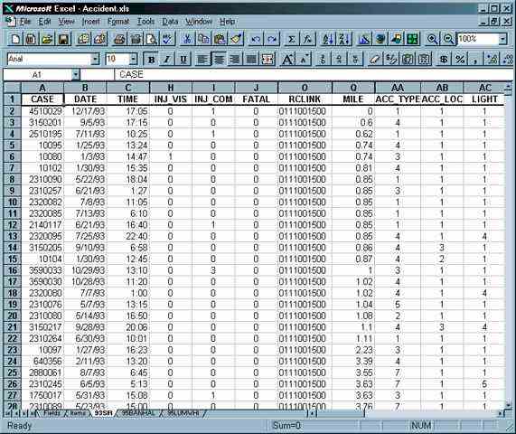
The FREQUENCY summarized the amount of each resource by type and link designation. To use the stream example again, each corridor link contained tens or hundreds of stream reaches. Some of those reaches were designated "Major," some "Minor" and some "Channel." Using FREQUENCY, ArcInfo automatically summed the total length of all stream reaches within each link that were attributed as "Major," "Minor" or "Channel." This frequency analysis was output to an ArcInfo INFO file, which was later exported into a Comma Separated Value (CSV) format readable by Microsoft Excel. The same procedure was used for all other linear features. For polygon features, the data were summed according to area (measured in square feet); for point data, the total count of each resource type by link was calculated. Roadway and Parkway statistics were calculated independently, and produced distinct CSV files.
The CSV files for each resource from a given alternative (i.e., Parkway or Roadway) were imported into an MS Excel spreadsheet. Some data from different FREQUENCY output files were imported into a single spreadsheet so that they could be added together, when appropriate. For example, the separate statistics for "Cropland" and "Pasture" from analysis of the Landsat land cover data were brought together in one spreadsheet so that they could be added together as a measure of "Agriculture." The spreadsheets also calculated acreage from the original square foot areal measurements output by ArcInfo.
Since otherwise comparable links might differ in length, a direct comparison of the absolute value of resource statistics was not always meaningful. For example, Parkway alternative Links A03 and A05 were functionally comparable (connecting Interstate 75 to a point roughly midway across Section 1 of the study area), but A05 was over three times as long as A03. The total number of stream reach feet in Link A05 was much larger (50,533) than in link A03 (about 22,000). However, when the number of stream reach feet in the two links was normalized by dividing each by the number of linear miles of corridor in each, it became evident that link A03 had the greater potential to affect stream resources (over 3,000 stream reach feet per mile of corridor for A03, vs. about 2,000 stream feet per corridor mile for link A05).
To perform the "per mile" normalization for all resource data, the Parkway and Roadway buffer coverages were overlaid on their respective centerline coverages, thereby assigning each portion of the centerline files to their appropriate corridor links. Using FREQUENCY, the length of each corridor link was ascertained. Those values were imported into the Roadway and Parkway spreadsheet models, and used to generate the appropriate normalized values: "Feet Per Mile" for linear resources, "Acres Per Mile" for polygon resources and "Sites Per Mile" for point data. The normalized data for roadway lanes were expressed as a percentage of total corridor length, rather than in units of "Feet Per Mile" or "Miles Per Mile." The resulting statistics were ranked in order from worst to best. The corridors at the top of the list thereby represented those with the greatest potential adverse impact; in any comparison of two otherwise functionally equivalent corridors, the one with the greatest potential impact could be identified.
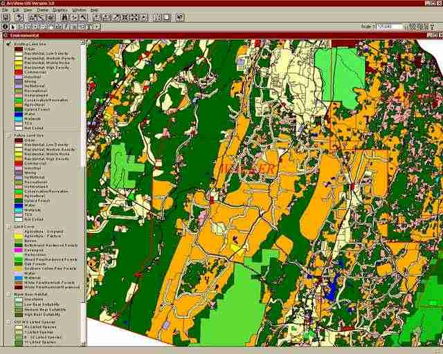
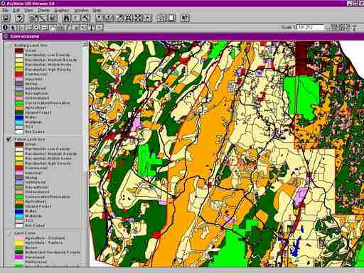
PHASE III: MORE CORRIDOR CHARACTERIZATION BY GIS
A number of cultural and natural resources factors were analyzed in Phase II as part of the process of identifying the four Phase III Corridors. To further differentiate the four remaining corridors, we identified factors contributing to the cost or benefit of any future road project. For example, the number of stream crossings encountered by a corridor not only provided a measure of relative environmental impact, but allow calculation of relative costs due to the number of bridges it required. Similarly, the number of accidents per mile on existing roads within a corridor provided a means to evaluate the savings in injuries, lives, medical costs and property losses possible through improvements that reduce accident frequency or severity. The GIS factors quantitatively analyzed during Phase III appear in Table 5.
|
TABLE 5 Factors Analyzed In Phase III GIS Corridor Evaluation Process |
||
|
Factor |
Description |
Sources |
|
Existing land cover and urban uses as identified from local government comprehensive plans, supplemented with land cover data from Landsat 30 meter satellite imagery. |
Existing Land Use data from Regional Development Centers; Landsat data from the Southern Appalachian Assessment; revisions by HDR Engineering. |
|
|
Future land cover and urban uses as identified from local government comprehensive plans, supplemented with land cover data from Landsat 30 meter satellite imagery. |
Future Land Use data from Regional Development Centers; Landsat data from the Southern Appalachian Assessment; revised to uniform land classification system by HDR Engineering. |
|
|
Stream Crossings |
Point locations at which stream centerlines crossed corridor centerlines, representing potential bridge sites. |
HDR Engineering analysis using GDOT hydrological coverage combined with Phase III corridor centerlines. |
|
Locations of automobile accidents for 1993 and 1995 within 300 feet of the centerlines for the alternative corridors. |
HDR Engineering analysis using GDOT 1993 and 1995 accident data, geocoded by HDR Engineering to mile marker locations via Dynamic Segmentation on GDOT road coverage. |
|
|
Slope Distance |
The linear distance along the nominal centerline of each link and/or corridor identified by the ASCS study team |
HDR Engineering analysis using USGS Digital Elevation Model data obtained from the Southern Appalachian Assessment. |
|
Vertical Profiles |
Elevation (in feet above Mean Sea Level) of corridor centerlines along the route of each corridor alternative. |
HDR Engineering analysis using USGS Digital Elevation Model data obtained from the Southern Appalachian Assessment. |
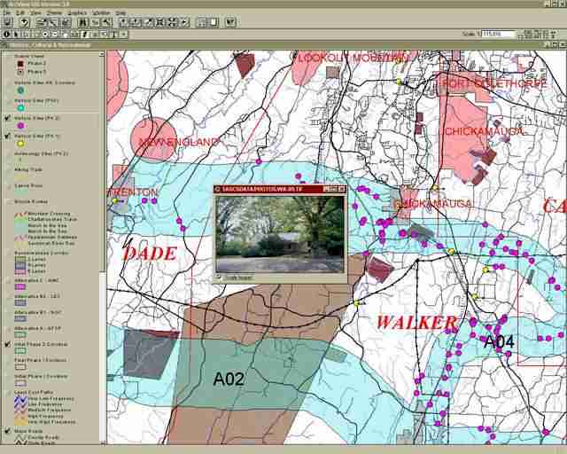
In addition to those factors, we continued to refine the cultural, historic and recreational database developed during Phases I and II with new information. Table 6 lists the data layers created or updated as part of that effort.
|
TABLE 6 Historic, Cultural & Recreational GIS Information Updated During Phase III |
||
|
Factor |
Description |
Sources |
|
Individual historic structures or locations. |
From surveys conducted by The Jaeger Company, supplementing data from the National Register of Historic Places, State Historic Preservation Office, and county surveys. |
|
|
Canoe Runs |
Rivers or streams identified as being suitable for recreational canoe use. |
Digitized into ArcView by The Jaeger Company based on various commercially available guide books. |
|
Hiking Trails |
|
Digitized into ArcView by The Jaeger Company based on various commercially available guide books. |
|
Bicycle Routes |
Proposed bicycle routes from GDOT’s Georgia Statewide Bicycle and Pedestrian Plan. |
GDOT bicycle routes mapped by The Jaeger Company and added to the GDOT roadway GIS database by HDR Engineering as of 10/97. |
|
Scenic Views |
Locations with potential as scenic overlooks or stops. |
Digitized into ArcView by The Jaeger Company based on field surveys. |
|
Archeological Potential |
Potential for archeological finds based on proximity to water and land slope. |
Map prepared by HDR Engineering based on model defined by New South Associates |
In most cases,
the data generated by the Phase III quantification effort were reported by corridor Link for each of the four alternative corridors still under study. The exception was vertical profile data, which were provided in x,y,z coordinate format for import into Microstation CAD software for further engineering analysis. Final selection of the Recommended Corridor relied heavily on cost/benefit ratios calculated, in part, on GIS-derived statistics. However, other sources of non-GIS information (such as the results of transportation network modeling) contributed significantly to the suite of factors evaluated by the Project Team in selecting the Recommended Corridor.
ALL PHASES: REPORTING & PUBLIC INVOLVEMENT
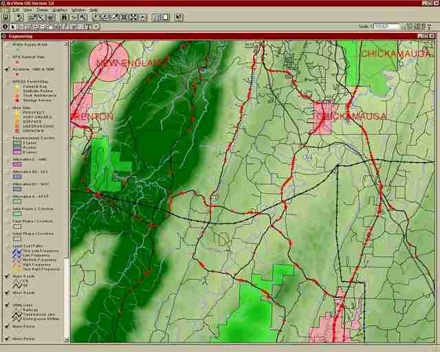
ArcInfo was used extensively to prepare map products for use in reports and public meetings.
Maps for Public Information Meeting (PIM) exhibits were plotted from an HP755CM Designjet and generally formatted for 24" x 36". These maps were mounted on foam core boards that could be hung from exhibit displays using Velcro fabric fastener tape. Report graphics were typically 11" x 17" versions of the 24" x 36" plots; report sized graphics were generated from the same map composition and GRA file by applying the appropriate scale factor in the POSTSCRIPT command. Using the same layout for both exhibits and report graphics saved considerable time. Report sized graphics were plotted on a continuous-tone color laser copier/printer using a Fiery interface.In addition to the static exhibits, the Project Team brought
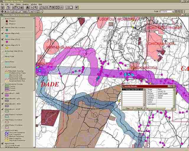
a desktop computer running ArcView 3.0 GIS to each Public Information Meeting loaded with the latest GIS data from the study. The ArcView database consisting of all the original coverages used in the Phase I least-cost path analysis, plus any additional coverages created during the course of the study. Using ArcView, a Project Team member could illustrate the study process, show the latest corridor concepts, and respond to queries from the audience. The PC was equipped with a 21" monitor, which was adequate for conducting demonstrations to groups of five or fewer people. A projection system was considered for use at the PIMs, but was rejected due to the difficulty of controlling lighting in large meeting rooms which must also accommodate other public meeting activities. Furthermore, we found that the intimacy provided by a small group around the monitor ensured better communication between the public and the ArcView operator.
CONCLUSIONS
This project illustrated the utility of using GIS as the central focus of a transportation planning project. In the initial phase, GIS provided the means to visualize the various constraints and suitability factors that must be balanced in the selection of transportation corridors. The least-cost path analysis provided a tool to assist the Project Team in organizing and evaluating the large amount of data available, and focus on corridors for further consideration. Throughout the project, the ability of GIS to quickly quantify all manner of impacts or corridor characteristics made it invaluable to the Project Team as they sought to differentiate between corridor alternatives. Map products prepared from the same data sets used in GIS analysis were useful to the Project Team as they evaluated corridor alternatives, and were just as valuable in explaining the Team's work to the public. Finally, the interactive use of ArcView in a public informational setting showed that GIS can help to further understanding of complicated issues by people as they contemplate the work of techical experts on matters that affect their community and their way of life.
ACKNOWLEDGMENTS
The following agencies provided spatial data or other assistance to the author which contributed enormously to the success of this project: The Southern Appalachian Assessment (Southern Man And Biosphere project), the Georgia Department of Transportation, the Georgia Department of Natural Resources, the North Georgia Regional Development Center, the Coosa Valley Regional Development Center, and the Georgia Mountains Regional Development Center. The principal members of the ASCS Project Team devoted the time and effort necessary to ensure that the full potential of GIS was realized for this study: David Cheeney, Mark Cheskey, Rusty Ligon and Tom Ziegler (HDR); Janet Harvey and Carl Spinks (Georgia DOT, Office of Planning); Dale Jaeger, Chet Thomas and Amy Kissane (The Jaeger Company); Theresa Hamby (New South Associates); Abraham Lerner (Transcore); and Douglas Bachtel (University of Georgia). Finally, I'd like to thank HDR Project Managers Margaret Ballard and Ken Anderson for their enthusiastic and continued support of GIS to transportation planning in this and other projects.
AUTHOR INFORMATION
Michael J. Gilbrook