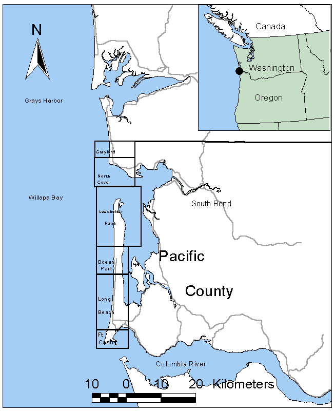
Figure 1. Map of Pacific County, Washington. Blocked areas indicate sub-regions used in the analyses.
The National Flood Insurance Reform Act of 1994 mandated that the Federal Emergency Management Agency (FEMA) conduct a statistically valid number of case studies to determine the feasibility of mapping erosion hazard areas in the United States coastal zone. FEMA funded the Washington State Department of Ecology to conduct one of these case studies in Pacific County. Pacific County is located north of the Columbia River and includes about 60 km of ocean shoreline. The overall objectives of the study were to map the current shoreline, calculated change rates, and project and plot the 60-year erosion hazard area with existing information from FEMA's Flood Insurance Rate Maps. In this paper the methods used to calculate these shoreline change rates are described.
During the study it was determined that about 626 structures larger than 5 by 5 m were within the projected 60-year (2055), 100 year flood zone. During the 1950 era to 1995 period rates of change within the County varied from 28.3 m/year of accretion to erosion of 27.0 m/year, with a mean rate of 0.9 m/year of accretion.
In this paper we will discuss and explain the methodology used to calculate shoreline change rates for Pacific County, Washington using ArcInfoTM and GridTM. This methodology is partially based on a white paper prepared by William Duffy and Stephen Dickson from the Maine Office of Geographic Information Systems, Augusta, Maine. Specifically, their methodology has been extended to deal with both accreting and eroding shorelines.
The methodology described here was developed to document and support a feasibility study being conducted by the Federal Emergency Management Agency (FEMA). The study was the result of increased developmental and population pressures in the United States coastal zone. These pressures, combined with chronic erosion problems in many areas, resulted in a effort in 1994 by the United States Congress to determine if it would be feasible to extend the Federal Emergency Management Agency's flood insurance program to cover areas at risk to erosion.
The National Flood Insurance Reform Act of 1994 mandated that FEMA conduct a representative study to determine the feasibility of mapping "60-year erosion hazard areas" (EHA) in the United States coastal zone. As part of the study FEMA identified several coastal counties on the Great Lakes and on the East, Gulf, and West Coast in which erosion hazard areas would be mapped. FEMA funded state or local agencies to perform these case studies. The Washington Department of Ecology was funded in 1996 to conduct one such case study for the ocean shoreline of Pacific County, Washington.
This study required that the Department of Ecology quantify shoreline change rates for Pacific County and use them to calculate and map the 60-year EHA for FEMA. However, accurate rates of change had never been calculated for the County. To complete the tasks required by FEMA, the Department of Ecology sought and obtained support from the U.S. Geological Survey and National Ocean Service, NOAA.
With the combined support of these federal agencies, the Department of Ecology was able to capture historical shorelines for entire Columbia River Littoral. This data was analyzed within the Departments geographic information system and, for the first time, accurate shoreline change rates obtained for the region.
The regional aspects of the study were funded jointly by the U.S. Geological Survey, Marine and Coastal Geology Program, and the Department of Ecology -with active participation of local communities and universities. This regional study, the Southwest Washington Coastal Erosion Study, extends 140 kilometers, from Tillamook Head, Oregon in the south to Point Grenville, Washington in the north. The regional study seeks to quantify both long-term (hundreds of years), mid-term (decades), annual, and seasonal (winter-summer) shoreline change rates and to construct a conceptual and predictive models of coastal change for the region (Gelfenbaum et al. 1997).
Previous regional studies (e.g., Phipps and Smith 1978, Phipps 1990) were hampered by a lack of accurate data from which to calculate mid- and long-term change rates. This study addressed this problem by deriving the historical shorelines directly from scanned Coast and Geodetic Survey (now the National Ocean Service) topographic sheets (T-sheets) and from orthophoto mosaics. Typically the accuracy of the derived shorelines were +/- 5 m or better. Details about the T-sheet conversion process are discussed in Huxford and Daniels, this volume. A paper describing the results and findings of this case study has been submitted to the Journal of Coastal Research (Kaminsky et al.).
Pacific County, Washington is located north of the Columbia River and includes 60 km of ocean shoreline (Figure 1). The County contains two coastal sections separated by the entrance to Willapa Bay: The Long Beach Peninsula section to the south and the North Cove or Cape Shoalwater section to the north. The ocean beaches are high-energy beaches consisting of fine-grained (~0.2 mm) Columbia River sand with slopes typically of 1:50 to 1:100.
Figure 1. Map of Pacific County, Washington. Blocked areas indicate sub-regions used in the analyses.
Pacific County has one of the most dynamic shorelines of any in the state, featuring both high erosion and high accretion rates. A maximum erosion rate of 45 m/year occured at North Cove in Willapa Bay. This erosion is caused by the northward migration of the tidal channel in the bay and has resulted in the loss of four lighthouses, a Coast Guard station, and a state highway since 1900. In spite of this, the County has a long-term accretion trend with C14 dating indicating a long-term accretion rate of about 0.4 m/year since the early 1700s to the 1870s. From the 1870 era to 1926 the mean accretion rate in the region had increased to 4.4 m/year, with localized accretion rates as high as 45 m/year occurring near the North Jetty (completed in 1911) on the Columbia River.
Nearly a century of high accretion rates has made the coast a favorable location for development. Shoreline progradation has allowed development to expand as it followed the movement of the shoreline westward. Concurrent with this accretion was the advent of the automobile and state and federal road networks. Via automobile, this strand of sand is only a two or three hour drive from Portland, Oregon and Seattle, Washington. This access has resulted in a 64% increase in housing growth rates, attributable to the construction of vacation homes, retirement homes, and tourist accommodations, compared to only a 15% increase in population between 1970 and 1990 (Boettcher 1991).
However, dam construction throughout the Columbia River basin during the mid-1900s has reduced peak river flows and may have reduced sediment discharges to the coast. Sherwood et al. (1991) has estimated that the total sediment discharge to the open coast has decreased by two-thirds since the early 1900s. Various indicators (e.g. a trend reversal to erosion at the North Jetty of the Columbia River) now suggest that a regional change in trend may be underway along the ocean coast of Pacific County.
A suite of software products were used in acquiring, processing, analyzing, and mapping the data. The primary software systems used were ArcInfoTM (for digitizing, mapping and analysis) and ERDAS Imagine TM (creation of orthophoto mosaics). The software was installed and run on a Sun Ultra 1 workstation with 20 Gbytes of dedication disk space.
Historical topographic sheets (T-Sheets) were obtained from the National Ocean Service (NOS) for the 1870 era, 1926, and the 1950 era (Figure 2). For the most part, the original T-Sheets are drawn at scales of 1:10,000 to 1:20,000 and have drafted accuracy’s of 3 to 6 m, respectively. The original T-Sheets from the 1870 era, 1926, and 1950 era were scanned by NOS at 400 dpi and provided to the Department of Ecology under a cooperative agreement. Ecology utilized ArcscanTM in combination with ArcView TM and several Avenue TM and Arc Macro Language (AML) scripts, to vectorize the shorelines from the T-Sheets. The digitizing process used was developed by the Department of Ecology and has been extended by NOAA's Coastal Services Center, Charleston, South Carolina.
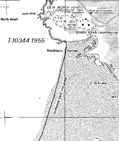
Figure 2. Example of part of a NOAA topographic sheet from 1955, sheet number T-10344.
This process resulted in the accurate digitizing of the historical shorelines from the T-Sheets at levels never before available. In most studies prior to 1997, coastlines derived from NOS T-Sheets were digitized from second or third generation copies using conventional digitizing methods –puck and table. In the process used here, the digitized line actually lies within the scanned line from the original document and the error, if any, is half the width of the line (0.79 m with a 1/32 inch line on a 1:20,000 scale map). Thus, errors due to the digitization and data conversion process are less than the error associated with the drafting method used by the original cartographer.
Detailed error analysis of the digitized shorelines from the 1926 and 1950 era T-Sheets has been conducted (Daniels and Huxford 1997). Concurrent with the scanning of the shorelines, cross hairs were digitized on all benchmarks shown on the original source maps. Published coordinates from the National Geodetic Survey for these marks were compared to the position of the benchmarks on the original maps, a mean error of +/-3.65 m was obtained. This meets NOS guidelines for fixed aids to navigation and objects charted as landmarks. The NOS guidelines are stricter than national map accuracy standards used by U.S. Geological Survey for 1:24,000 maps. Because of this, it can be assumed that the mapped shorelines meet published NOS guidelines (Shalowitz 1964) and are very accurate depictions of the shoreline as it existed during the survey. This also indicates that the registration and rectification process has corrected for any shrinkage or warping of the original paper or cloth maps that may have occurred during scanning or during storage over the last 40 to 120 years.
The contemporary shoreline was obtained from photography flown in August and September of 1995 by NOAA. The 1:12,000 scale photography was flown under a variety of tidal conditions with tidal elevations varying from –0.46 m to 2.74 m mean lower low water (MLLW).
The diapositive originals were scanned using an Agfa Horizon Ultra scanner at 600 dpi (0.5 m by 0.5 m). This resolution was selected based on two factors, the expected maximum accuracy in determining a shoreline and the desire to minimize file size (22 Mbytes at 600 dpi, 122 Mbytes at 1,200 dpi). Over 100 photos were scanned and archived to CD-ROM.
ERDAS ImagineTM and OrthomaxTM were used to georeference, orthorectify, and mosaic the photography. The final mosaics covered the entire ocean shoreline of Pacific County. Most of the study area had mean locational errors of 1.5 to 3 m. In Leadbetter Point (see Figure 1), identifiable pass points and ground control points were limited due to the flat undeveloped topography, resulting in higher mean error of 5 to 8 m.
The shoreline, taken to be the average high water line, and vegetation line were digitized in ArceditTM utilizing a customized AML designed for that purpose. The digitizing operator used visual cues in a manner similar to those employed by the NOS topographers to determine the boundary between which an average high tide often reaches and a higher high tide reaches less frequently. In general, the average high water line (AHWL) is taken to be "on the Pacific Coast, with two high tides of unequal height, the line … between these lines. If only one line of drift exists the line is slightly seaward of such a drift line. The line is not considered to be the storm high water line" (Shalowitz 1964). The principal cues used to determine the location of this line include the following:
These five cues are used while heads-up digitizing within ArceditTM. The heads up digitizing method allows zooming of up to 1:1 as the operator resolves the AHWL. Concurrent with the digitizing process the operator assigned quality assurance codes to the digitized AHWL, indicating their certainty in locating the line. Figure 3 shows a 1995 orthophotograph with the digitized AHWL in blue and the vegetation line in red, along with the 1955 shore and vegetation line (orange). The 1955 coastline was derived from the NOS T-Sheet shown in Figure 2.
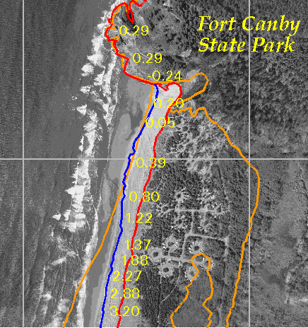
Figure 3. Comparison of the digitized 1995 AWHL (blue) and vegetation line (red) with the shoreline and vegetation line (orange) from 1955 obtained from a NOS T-Sheet.
A detailed analysis of this uncertainty (in locating the AHWL) has not been conducted, although it may be large considering the mild beach slopes and high tide ranges in the study area. However, this digitizing method is similar to the methodology used by NOS for the original T-Sheets. It is currently estimate that the error is on the order +/-10 m, with increased experience of the operator reducing this error to +/-5 m.
The AML program used for the analysis is designed to automate the calculation of erosion and accretion rates (accretion is negative, erosion positive). The complete text of this program is contained in the Appendix. This AML uses the form shown in Figure 4 to obtain the following: cover name of the reference shoreline, year of reference shoreline, name of the old shoreline, year of old shoreline, name of the mask coverage to be created, name for the resulting arc coverage’s with the calculated change rates, and the name and year for which a future shoreline will be predicted. The two input shorelines are line coverage’s. The mask coverage is a polygon coverage and is created by this AML and user modified within ArceditTM. The change rate and future shoreline coverage’s are created by the AML and contain line/arc attributes.

Figure 4. The form used to obtain the input and output coverage names used by the AML.
After the form is completed the AML checks for and deletes any temporary files in the current workspace that may have been created by a previous iteration of the program. On completion of the "cleanup" procedure the erosion calculation procedure begins.
The erosion procedure involves a multi-step process. First, the reference and old shoreline are converted into grids with the LINEGRID command. The shoreline year, an item within each shoreline coverage attribute file (AAT), is used as the value item. The cell size used for the resulting grids was 1 m. This cell size value is set as a global AML variable at the top of the program. The old shoreline coverage is then copied into the mask coverage.
ArceditTM is started with the edit cover set to the mask cover and the edit feature set to arc (line). The operator digitizes a box that just touches the edges of the coastline. This box should be large enough to cover the extent of both the reference shoreline (used as a background coverage) and the old shoreline. Polygons are then built using the clean command within ArceditTM, the polygons on the landward side of the shoreline are given a code of 1 and the seaward polygons are given a code of -1. POLYGRID is then run to convert the mask coverage into a grid (named GRIDMSK) using the polygon code as the value item.
On completion of the grid conversion process, GridTM is started to perform computationally intensive operations. Within GridTM several temporary grids are created. The two primary ones are named GOLDYR and OLDDIST. GOLDYR contains a grid with NO-DATA values for all cells except those cells that fall on the old shoreline. These cells have a value equal to the shoreline year.
Grid OLDDIST is created by calculating the euclidean distance, using the EUCDISTANCE procedure, from the old shoreline contained within GOLDYR. Euclidean distance is calculated from the center of the source cells (i.e., cells with year values for the old coastline) to the center of the surrounding cells. Thus, the output of this process is a cost surface, where the "value" is the distance from the nearest cell that had a portion of the old coastline within it (Figure 5). This process produces the true distance, not a cell distance. The resulting grid, OLDDIST, contains floating-point distance values.
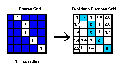
Figure 5. Example of the input (GOLDYR) and output grid (OLDDIST) produced by the EUCDISTANCE procedure in GridTM.
The output change values are stored in an integer grid. The change grid is calculated by taking the reference grid (shoreline) and asking the following question on a cell by cell basis:
Change Grid = CON ( GREF eq YEAR1, INT ( OLDDIST * GRIDMSK * 10 ), ) ,
where CON is a GridTM if-then-else function, GREF is the reference shoreline grid, and YEAR1 is the year represented by the reference shoreline. The value of the equation "OLDDIST * GRIDMSK * 10" is returned and stored in the change grid if the expression, GREP equals YEAR1, evaluates to true. If the expression is false the change grid is assigned a NO-DATA value for the given cell. The value assigned to the change grid, under the true condition, was multiplied by 10 to overcome rounding problems that occurred when the floating-point grid was truncated using the INT function. After completion of the change grid, GridTM is terminated.
The change grid is then converted back to a vector format using the GRIDLINE procedure with the nothin, nofilter, and round options and built with the BUILD procedure. The resulting coverage has one data variable, named VALUE, that contains the total accretion or erosion that has occurred between the reference shoreline and "old" shoreline. The RATE variable is then added to the coverage and TABLES started (TABLES is an attribute data manager subsystem of ArcinfoTM).
Within TABLES the VALUE variable is divided by ten to correct for the conversion to integer that was done within GRIDTM. The RATE variable is destined to contain the actual change rate in m/year and is calculated as follows:
RATE = VALUE / ((YEAR1 – YEAR2 ) + 1)) ,
where YEAR1 and YEAR2 are the years represented by the reference shoreline and old shoreline, respectively. Thus, completing the change rate coverage (In the future, this calculation will be modified to take into account the month as well as the year of the shoreline.).
To allow for further automation of the analysis process a second version of the change rate coverage is created. The arcs in the completed change rate coverage are split at one-meter intervals using the DENSIFYARC procedure. This results in a second line coverage with the same information as the first coverage. In addition, the coverage has been modified so that all line segments are only one meter long. A TRANSECT variable was then added and line segments that are about 50 m apart are given a value of 1, all others are 0.
The procedure used to assign the TRANSECT value is based on a modulus (MOD) function. Since TABLES does not support a MOD function, one was simulated as follows. Two temporary variables were added to the densified change rate coverage. The first, TRANINT, was defined as an integer and the second, TRANFLT, as a real (floating point number). The line segment numbers assigned within ArcinfoTM were then divided by 50 and assigned to each variable. Since TRANINT was an integer, the remainder from this division process was truncated. The line segments for which the attribute values of TRANINT and TRANFLT were equal were then selected and the TRANSECT variable set. The transect spacing calculated using this method may be modified to allow for spacing at intervals other than 50 m (e.g., 100 m).
This AML allows users to project a future shoreline based on the change rates obtained during the analysis. The future coastline is projected based on linear interpolation of the change rates. This is accomplished by adding the following three variables to the densified change rate coverage: FUTURE, ABSFUT, and DISS. After adding these variables TABLES is started. The FUTURE variable is calculated and contains the total distance of accretion or erosion that will occur from the reference year (YEAR1) to the selected future year (YEAR3). ABSFUT contains the absolute value of FUTURE. DISS is calculated by dividing ABSFUT by 10. This last variable was used in conjugation with the DISSOLVE command with the line option to obtain a simplified shoreline prior to running the BUFFER procedure.
The BUFFER procedure takes the simplified coastline produced by the DISSOLVE command and buffers it based on variable ABSFUT with the flat, full options. The simplified shoreline and the buffer polygons are then appended using the APPEND procedure with the arc, none options. Topology for the future shoreline coverage is then created using the CLEAN procedure.
ArceditTM is started with edit coverage set to the future shoreline and the edit feature set to arc (line). The operator is then presented with a display (shown in Figure 6) in which the reference coastline is color-coded indicating if each particular line segment is accreting (purple) or eroding (yellow). If a particular line segment shows erosion, then the seaward buffer line would be selected and deleted (along with the reference shoreline). Conversely, if the reference shoreline indicated accretion, then the landward buffer and shoreline line would be deleted.
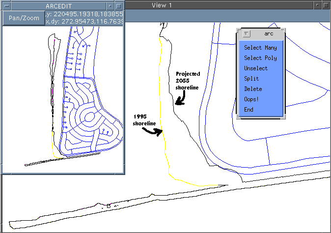
Figure 6. The Arcedit display used to update the projected future coastline coverage.
The overall objectives of the study were to map the current shoreline, calculate change rates, and project and plot the 60-year erosion hazard area along with existing information from FEMA's Flood Insurance Rate Maps. During the study it was determined that about 626 structures larger than 5 by 5 m were within the projected 60-year, 100 year flood zone. In the 1950 era to 1995, rates of change varied from 28.3 m/year of accretion to erosion of 27.0 m/year. The mean rate for the region was 0.9 m/year of accretion.
The calculated change rates for the study area are shown in Figure 7 (accretion is negative, erosion positive). The rates shown were obtained at 1 kilometer intervals. The highest accretion rates occurred prior to the 1950s at Fort Canby (near kilometer 61 to 64), at the North Jetty on the Columbia River. A change in trend to erosion occurred at Fort Canby after 1950. Note the distance over which the construction of the North Jetty (completed in 1911) impacted the region –20 kilometers of shoreline to the north of the jetty experienced a significant increase in accretion. The only area unaffected was located at kilometers 59 and 60, the location of a prominent rocky headland.
Conversely, the highest erosion rates occur at the north entrance of Willapa Bay near North Cove (kilometer 9 to 13). In this area over two linear miles of land have been lost since 1871. This erosion is due to the northward migration of the northern tidal channel (Terich and Levenseller 1987). Maximum channel depth has also increased, from about 8 m in 1871 to a current depth of 20 m. This migration may have been forced by the filling and partial closure of the southern tidal channel from sediment inputs from Leadbetter Point.
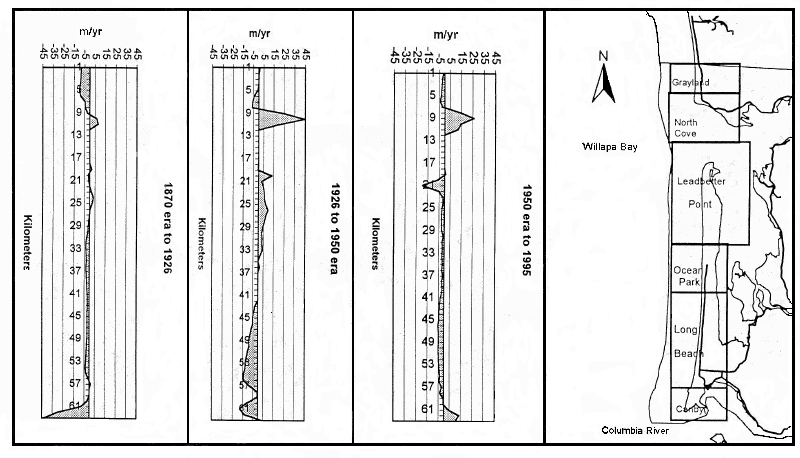
Figure 7. Plot of shoreline change rates for Pacific County, Washington. Note that no data are available for kilometers 38 to 42 during the 1926 to 1950 period. The data for this region in the period 1950s to 1995 actually represents the 69-year period 1926 to 1995.
In this paper an AML program used to calculate historical coastline change was described. Coastal change studies have traditionally quantified change rates at transects that may be spaced at 50 m (e.g., in Florida) to as far apart as tens-of-kilometers. Determination of the orientation to be used for transects is problematic on any nonlinear coastline, as transects only show the change along the line.
The methodology used here obtains a change rate for every meter-long line segment of the shoreline. The change rate is based on the shortest distance between the reference shoreline (current coast) and old shoreline, for each line segment in the reference shoreline. This methodology minimizes the two major limitations with traditional transect based studies. Firstly, the change values calculated are the shortest distances between the two shorelines (direction is not considered). Secondly, transect spacing is not a limiting factor in the analysis and modeling of the data, as change values may be obtained anywhere on the coast at the click of a button.
This does not say that the traditional transect concept is not useful. In our study the use of transects provides an opportunity to easily graph and perform regional comparisons of the data. However, this methodology insures that the transect spacing used for a particular application is not limited by the available information.
This research was partially funded by FEMA under contract EMW-96-CA-0222. The support of the U.S. Geological Survey and the National Ocean Service, NOAA, for assisting in hardware, software, and data acquisition are greatly appreciated.
Boettcher, S.B. 1991. Population and Development Trends in Washington State’s Coastal Zone. White paper, Shorelands and Coastal Zone Management Program, Department of Ecology, Olympia, WA.
Daniels, R.C. and R.H. Huxford. 1997. NOAA, Topographic Sheets: Error Assessment of Vectorized Lines Based on Coordinates from NGS Survey Markers. White paper, Coastal Monitoring and Analysis Program, Department of Ecology, Olympia, WA.
Duffy, W. and S.M. Dickson. Using Grid and Graph to Quantify and Display Shoreline Change. White paper, Maine Office of Geographic Information Systems, Augusta, ME.
Gelfenbaum, G., Kaminsky, G.M., Sherwood, C.R., and C.D. Peterson. Southwestern Washington Coastal Erosion Workshop Report. Open-File Report 97-471, U.S. Department of the Interior, U.S. Geological Survey, Washington, DC.
Huxford, R.H. and R.C. Daniels. This Volume. Historical map recovery using multiple integrated Esri programs. Proceedings, 1998 Esri Users Conference, San Diego, CA.
Kaminsky, G.M., R.C. Daniels, R.H. Huxford, D. McCandless, and P. Ruggiero. Submitted 12/1997. Mapping erosion hazard areas in Pacific County, Washington. Journal of Coastal Research.
Phipps, J.B. 1990. Coastal accretion and erosion in Southwest Washington, 1977-1987. Publication 90-21, Shorelands and Coastal Zone Management Program, Department of Ecology, Olympia, WA.
Phipps, J.B. and J.M. Smith. 1978. Coastal accretion and erosion in Southwest Washington. Publication 78-12, Department of Ecology, Olympia, WA.
Shalowitz, A.L. 1964. Shore and Sea Boundaries. Publication 10-1, U.S. Department of Commerce, Coast and Geodetic Survey, Washington, DC.
Sherwood, C.R., D.A. Jay, R.B. Harvey, P. Hamilton, and C.A. Simenstad. 1990. Historical changes in the Columbia River Estuary. Progress in Oceanography 25:299-352.
Terich, T.A. and T. Levenseller. 1987. The severe erosion of Cape Shoalwater, Washington. Journal of Coastal Research 2:465-477.
Phone: (360) 407-6427
E-mail:
/* AML change.aml created: 3/28/1997
/* by Richard C. Daniels
/*    CMAP, Shorelands & Environmental Assistance
/*    Department of Ecology
/*    Olympia, WA 98504-7600
/*
/* Modified 3/16/1998
/* Remove ap command in arcedit session within the futurecoast procedure.
/* Reorder the procedures to better reflect the flow of control within
/* the program.
/*
/* Modified 2/25/1998
/* To allow multiple edits of the mask coverage before using POLYGRID.
/* to covert the mask polygons to a grid for use in the change analysis.
/*
/* This aml is designed to automate the calculation of erosion/accretion rates
/* between an old shoreline and a newer reference shoreline (e.g., 1995).
/* The initial portion of this AML is based on a manuscript entitled "Using grid
/* and graph to quantify and display shoreline change" by William Duffy and Stephen M.
/* Dickson (http://apollo.ogis.state.me.us/projects/p074.htm) and has been
/* extended to deal with both accreting and eroding shorelines.
/*
/* After the aml calculates the change from the old to reference shoreline
/* the user is given the option of creating a predicted future shoreline using
/* the buffer command. The future shoreline is measured from the reference
/* shoreline based on a given year in the future.
/*
/* Program MAIN
&sv cellsize = 1
&terminal 9999
&severity &warning &ignore
&severity &error &ignore
&popup change.info
&menu change.menu
&if [exists %.mask% -cover] or [exists gridmsk -grid ] or [exists gold -grid] or ~
    [exists gref -grid] or [exists %.change%_c -cover] or ~
    [exists %.mask% -cover] or [exists %.change% -grid]  &then &call cleanup
&if %.quit% = 0 &then &do
                      &call erosion
                      &call futurecoast
                      &end
&call cleanup
&return

/* Calculate the coastline for a future year
&routine futurecoast
/* &return    May be disabled if not required for the given analysis
&type Creating %.future% with the future coastline for %.year3%.
additem %.change%_den.aat %.change%_den.aat future 8 8 i
additem %.change%_den.aat %.change%_den.aat absfut 8 8 i
additem %.change%_den.aat %.change%_den.aat diss 8 8 i
additem %.change%_den.aat %.change%_den.aat symbol 8 8 i
tables
select  %.change%_den.aat
calc future = rate * ( ( %.year3% - %.year1% ) + 1 )
calc absfut = future
reselect future <0
calc absfut = ( future * -1 )
calc symbol = 6
nsel
calc symbol = 7
aselect
calc diss = absfut / 10
q
dissolve  %.change%_den %.change%_simp diss line
additem %.change%_simp.aat %.change%_simp.aat absfut 8 8 i
additem %.change%_simp.aat %.change%_simp.aat symbol 8 8 i
tables
select %.change%_simp.aat
calc absfut = diss * 10
q
buffer %.change%_simp %.change%_buff absfut # # # line flat full
build %.change%_buff line
dropitem %.change%_simp.aat %.change%_simp.aat diss
dropitem %.change%_simp.aat %.change%_simp.aat absfut
append %.future% notest features
%.change%_buff
%.change%_simp
end
clean %.future% # # # line
arcedit
display 9999
edit %.future% arc
/* Coastrd is a road coverage used to provide locational informationj
backc $HL/lib_cover/coastrd 4
backc %.change%_den
backsymbolitem %.change%_den arc symbol
backenv arc
drawenv arc
&label top3
draw
&type Select the buffer and coastlines from %.future% to be deleted.
&sv action = [menu change_ed.menu -sidebar]
&if %action% eq 0 &then &do
                        select many
                        drawselect
                        &end
&if %action% eq 1 &then &do
                        select poly
                        drawselect
                        &end
&if %action% eq 2 &then unselect all
&if %action% eq 3 &then &do
                        sel one
                        split
                        &end
&if %action% eq 4 &then delete
&if %action% eq 5 &then oops
&if %action% eq 6 &then &goto end
&goto top3
&label end
quit yes
&type %.future% creation complete.
kill %.change%_simp all
kill %.change%_buff all
&return

/* Calculate the accretion or erosion rates between the "old" and reference shoreline
/* Convert vectors to GRID
&routine erosion
&type Rasterizing lines.
linegrid %.refc% gref year
%cellsize%
y
nodata
linegrid %.oldc% gold year
%cellsize%
y
nodata
copy %.oldc% %.mask%
&type Starting Arcedit.
arcedit
display 9999
edit %.mask% arc
drawenv arc on
nodesnap closest 100
arcsnap on 100
mapex %.refc% %.mask%
backc  %.refc% 3
backenv arc
/* Editing of mask coverage
&label top
    draw
   &type Digitize a box that just touches the edges of the coast.
   add
   clean
   draw
   editf poly
   drawenv poly
   &type Select the land polygon (to test the closure of the box).
   draw
   select many
   drawsel
   &type Select the sea polygon.
   unselect all
   draw
   select many
   drawsel
   editf arc
/* Small holes in the source coastline may need additional editing.
/* This is not known until this point. The user is given the option to
/* continue to edit the mask coverage prior to saving.
  &sv loop  = [response '(1) Continue to edit or hit return to continue' 0]
  drawenv poly off
  draw
&if %loop% = 1 &then &do
                           edit %.mask% arc
                           &goto top
                           &end
&type Cleaning the coverage.
clean
&type Saving the coverage.
save
q
&type Adding the "code" item to %.mask%.
additem %.mask%.pat %.mask%.pat code 4 4 i
&type Restarting Arcedit to update code.
arcedit
edit %.mask% poly
drawenv poly
&type Select the polygons landward of the coastline.
&label looP2
   draw
   select many
   &sv loop  = [response '(1) Unselect and start over or hit return to continue' 0]
   &if %loop% = 1 &then &do
                            unsel all
                           &goto looP2
                           &end
/* erosion is positive
calc code = 1
nselect
/* accretion is negative
calc code = -1
save
q
polygrid %.mask% gridmsk code
%cellsize%
y
&type File and grid creation complete. Starting Grid.
&call dogrid
gridline %.change% %.change%_c data nothin nofilter round value # %cellsize%
build %.change%_c line
additem %.change%_c.aat %.change%_c.aat rate 8 8 f 2
&call filter
&type Coverage %.change%_den has been completed and contains the
&type per year change rate and total change value from %.year2%
&type to %.year1% for 1 meter long arcs. The variable "transect"
&type has been added to the coverage with a value of 1 for line
&type segments that are located at 50 m interals.
&return

/* Simplify line produced by gridline
&routine filter
tables
select %.change%_c.aat
/* Divide by ten to correct for conversion to integer in grid
calc value = value / 10
calc rate =  value / ( ( %.year1% - %.year2% ) + 1 )
q
densifyarc %.change%_c %.change%_den 1 arc
build %.change%_den arc
additem %.change%_den.aat %.change%_den.aat tranflt 8 8 f 2
additem %.change%_den.aat %.change%_den.aat tranint 8 8 i
additem  %.change%_den.aat %.change%_den.aat transect 8 8 i
tables
select %.change%_den.aata
/* Divide by 50 m to flag line segments that are about 50 m apart.
/* Could divide by 100, for example, to flag transects at about 100 m intervals.
calc tranflt = %.change%_den# / 50
calc tranint = %.change%_den# / 50
reselect tranint eq tranflt
calc transect = 1
q
dropitem %.change%_den.aat %.change%_den.aat tranint
dropitem %.change%_den.aat %.change%_den.aat tranflt
&return

/* Grid overlays to calculate change from old to ref coastline
&routine dogrid
grid
setcell %cellsize%
setwindow minof
goldyr = con ( gold eq %.year2% , gold)
kill gold all
olddist = eucdistance ( goldyr )
%.change% = con ( gref eq %.year1%, int ( olddist * gridmsk * 10 ) )
q
kill goldyr all
kill olddist all
&return

/* Delete temp files created during the analysis
&routine cleanup
&type
&type Deleting temp files.
kill gref all
kill gold all
kill gmsk all
kill gridmsk all
kill %.mask% all
kill %.change% all
&type Normal end.
&return
This aml is designed to automate the calculation of erosion rates between a old shoreline and a reference shoreline (i.e., 1995). The initial portion of this AML is based on a manuscript entitled "Using grid and graph to quantify and display shoreline change" by William Duffy and Stephen M. Dickson (http://apollo.ogis.state.me.us/projects/p074.htm) and has been extended to deal with both accreting and eroding shorelines. After the aml calculates the change from the old to reference shoreline the user is given the option of creating a predicted future shoreline, measured from the reference shoreline, for XX years into the future. You will be asked to enter the names of the following: old shoreline coverage, reference shoreline coverage, mask coverage. The mask coverage will be created on-the-fly in arcedit based on the old shoreline data and with the reference shoreline as a back cover. Clickto continue.
7 change.menu
Select and enter the coverage names to be used.

Reference Shoreline  %cover1
Year of reference shore %year1

Old Shoreline        %cover2
Year of old shore %year2

Name of mask coverage
(to be created)      %mask

Change cover
(to be created)      %change

Future cover
(to be created)      %future
Year of future shore %year3

             %apply             %cancel


/* Field Definitions
%cover1 input .refc 20 required cover
%year1 input .year1 20 required integer
%cover2 input .oldc 20 required cover
%year2 input .year2 20 required integer
%mask input .mask 20 required character
%change input .change 20 required character
%future input .future  20 required character
%year3 input .year3 20 required integer
%apply button Apply &sv .quit = 0; &return
%cancel button Cancel 'Abort' &sv .quit = 1; &return
2 Selection Menu
'Select Many' 0
'Select Poly' 1
Unselect 2
Split 3
Delete 4
Oops! 5
End 6