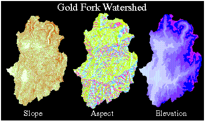
Figure 1. Examples of Univariate Geographic Layers for Predicting Site Potential.
Stephen P. Warren
One of the primary barriers to effective
implementation of ecosystem management across forested landscapes
is the inability to apply ecological land classification systems
because of the lack of ecologically based map information. One
such ecological land classification system is the habitat type
classification for forest types. A habitat type, the basic unit
of site potential, is an integrated expression of the physical
and biophysical environment. A habitat type reflects the combined
effects of climate, topography, soils and other environmental
values which occur along an environmental gradient of warm moist
conditions to cool dry conditions. With the capabilities of ArcInfo
Grid GIS, this environmental gradient can be modeled to predict
habitat type classes and map broad landscapes.
Implementing effective ecosystem management approaches and analysis at larger spatial scales requires the development of appropriate ecological classification systems that characterize and describe ecosystems. Since 1994, Boise Cascade Corporation has been involved in an ecosystem management project with multiple landowners for the purpose of developing an ecosystem strategy for the 5.8 million acre Idaho Southern Batholith landscape. As a part of this strategy, Boise Cascade's Idaho Ecosystem Management Project implemented an existing ecological land classification system known as the Ecosystem Diversity Matrix (Haufler 1994) to quantify ecological diversity in the Idaho Southern Batholith landscape. As a ecological land classification system, the matrix provides the foundation for ecosystem management planning and represents the primary tool for quantifying existing forest landscape conditions, describing historical conditions, and developing targets for desired future conditions.
The Ecosystem Diversity Matrix incorporates another ecological classification system known as a habitat type classification. Habitat type classification systems describe the site potential of the land as expressed through combinations of environmental interactions which determine the vegetation found on any given site (Daubenmire 1968). In 1981, Steel et al. developed a forest habitat type classification system describing potential or climax vegetation for west-central Idaho. In this classification system Steele et al. identified 56 forest habitat types for the Idaho Southern Batholith. These 56 habitat types were then reclassified or categorized into 11 habitat type classes by Steele to represent more operationally functional units for describing site potential. These eleven classes reclassified from the 56 habitat types were combined based on similar successional response in terms of species composition, structure and succession for the range of disturbance regimes associated with each class. For example, all dry to extremely dry ponderosa pine habitat types were reclassified into a individual habitat type class describing the Xeric Ponderosa Pine Habitat Type Class. Once the 56 habitat types were reclassed into the eleven habitat type classes, they were then inserted into the Ecosystem Diversity Matrix and used to characterize and quantify the number and amount of different site potentials or habitat type classes represented in the ecological communities present in the Idaho Southern Batholith landscape.
Habitat type classification systems such as the forest habitat type classification in west-central Idaho have become a proven tool for land management decision making, research and forest planning. However, as with many other field research developed classification systems, they are implemented in the field with a dichotomous key using vegetative indicator species to classify each site on a sample plot basis only. In fact, over the course of its use in the past 20 or more years, there has been very little progress in moving away from the point sample based method to a GIS mapping approach for delineating habitat types. Because most of the available habitat type information has been primarily collected on a plot or point basis, the majority of the landscape in west-central Idaho has never been mapped for the 56 available habitat types nor for the 11 habitat type classes defined in the Ecosystem Diversity Matrix.
This paper describes a geographic information
system (GIS) ArcInfo application to predict and map habitat type
classes in west-central Idaho to support the implementation of
an ecological land classification system for the Idaho Southern
Batholith. The application methodology relies on the conceptual
theory of environmental and identifies new geographic information
system layers that reflect the combined effects of climate and
topography and other thematic information to spatially predict
and map 11 habitat type classes.
After a preliminary review of other existing
or past efforts in Idaho and other parts of the Pacific Northwest
to try to use GIS to map site potential, potential vegetation
and/or habitat types or habitat type classes it was concluded
that most of those efforts relied on univariate or single variable
geographic layers to predict site potential. In addition, most
of the identified efforts used GIS layers or coverages which were
often derivatives of digital elevation models which describe characteristics
about the topography of the landscape. The three most commonly
used univariate layers in mapping site potential or habitat types
were slope, aspect and elevation, see figure 1. Once these layers
were generated for a specific site, the next step was to develop
logically structured mutually exclusive spatial queries describing
combinations of slope, aspect and elevation values to predict
where on the landscape certain habitat type classes would most
likely exist.
Figure 1. Examples of Univariate Geographic Layers for Predicting
Site Potential.
While most of these habitat type or potential vegetation mapping efforts have included other additional geographic input layers with varying spatial logic prediction methods, what has been learned most in reviewing these other efforts is that they haven't always worked toward developing geographic input layers that describe environmental interactions or combinations of geographic input layers describing environmental conditions. This subjective conclusion is based purely on a limited set of observations and is in no way meant to discredit the efforts of others pursuing this same endeavor. However, based on this observation and in this effort to discover the range of environmental patterns and conditions that exist across the landscape for predicting and mapping site potential via habitat type classes, a number of multivariate integrated geographic information layers were developed to help better understand the spatial relationships associated with habitat type classes on the landscape that were also observed in the field.
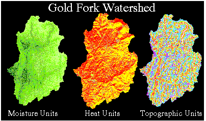
Newly created and developed GIS information
layers describing environmental interactions are referred to as
plant/environmental layers. In figure 2, a few examples of the
plant/environment interaction layers are illustrated like available
moisture units, heat units and relative topographic position units.
While each one of these layers have been constructed with a different
set of logical definitions, the intent in the development of each
interaction layer was to describe the kind of physical environmental
conditions that determine the life history requirements of different
ecological communities and their associated site potential. In
other words, these efforts were a first attempt to create geographic
information system layers that best describe the environmental
conditions that support the 11 identified habitat type classes.
Figure 2. Examples of Multivariate Environmental Interaction Layers for Predicting Site Potential.
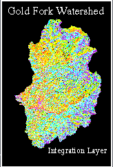
As integrated geographic layers were developed
integrating as many different information system layers as possible,
the multivariate integrated input layers were then compared with
mapped habitat type class polygons that had been field mapped
in the west-central Idaho in the mid to late 1970's. Visual examinations
were then made between the newly developed interaction layers
and mapped polygons of habitat classes to look for and identify
coincident patterns. Overtime, it became increasingly apparent
that the patterns generated by integrating the different single
variable layers into a set of multivariate environmental interaction
output layers seemed to aligned themselves quite reasonably to
the mapped polygons of habitat type classes. Figure 3 illustrates
one of the integrated environmental input layers that resulted
in map patterns that matched most closely to mapped polygons of
habitat type class data. This layer referred to as an integrated
environmental layer was constructed by integrating or combining
the separate layers of slope, aspect, elevation, ambient air temperature,
mean annual precipitation, solar radiation, and topographic moisture.
Figure 3. Example of Environmental Integration Layer.
While the integration layer development
demonstrated promise both visually and intuitively, most of the
integration layers had a very limited scientific basis for supporting
the combination and integration of these univariate input layers
into combined multivariate layers. In addition, it still wasn't
evident how these interaction layers could then be used to support
the development of spatial relationships for predicting habitat
type classes. As a result, instead of continuing to pursue the
development of more integrated layers, it was determined that
there was a need to return to a more foundational scientific basis
for developing appropriate geographic layers and to identify a
more defensible methodology for combining those information layers
to predict habitat type classes. The investigation next turned
to the conceptual theory behind habitat type classification to
determine where and how to proceed. In reviewing the habitat type
classification concept, a more scientific basis and methodology
for developing spatial habitat type relationships was identified
as well as how to incorporate some of the earlier developed environmental
integration layers.
The ArcInfo Grid mapping tool methodology that is currently being used and proposed for this application is one that attempts to describe where in real landscape space different habitat type classes occur along an environmental gradient. This methodology has been adapted from the original habitat type concept where habitat types or habitat type classes can be found along an environmental gradient of warm dry to cool moist conditions (Daubenmire 1968). Figure 4 illustrates how different habitat type classes are oriented along this environmental gradient. For example, in figure 4, Habitat Type Class A represents a site potential which is on the extreme warm, dry end of the environmental gradient continuum while Habitat Type Class D is on the extreme cool moist side of the environmental gradient. In between these two extremes, other habitat type classes occur based on the environmental conditions and resources that support these site potentials.
This method further builds upon the concept of environmental gradients by dividing the gradient into two primary axes, a temperature axis which describes warm to cool environmental conditions and a moisture axis which describes dry to wet conditions, see figure 5. With these two primary axes, habitat type classes can be delineated graphically in two-dimensional space to display the range of landscape conditions where different habitat type classes will be found. In a way, this graphical tool illustrates how along an environmental gradient of warm dry conditions to cool moist conditions moisture will compensate for temperature and temperature will likewise compensate for varying levels of moisture to provide the primary environmental conditions that determine where different habitat type classes might exist on the landscape.
Figure 4. Habitat Type Class Environmental
Gradient Concept.
| Habitat Class A | Habitat Class B | Habitat Class C | Habitat Class D |
(warm,dry)----------------EnvironmentalGradient----------------(cool,moist)
In figure 5, the range of habitat type
class conditions for each habitat type class are identified or
defined in space by a honeycomb like geometric shape. This shape
illustrates where each habitat type class is oriented within this
environmental gradient and each side of the geometric shape represents
the ecotones or ecological transitions between different habitat
type classes. In a way, this graphical tool illustrates how along
an environmental gradient of warm dry conditions to cool moist
conditions where more or less moisture will compensate for more
or less temperature and in part determine where in real space
a habitat type class might exist. It is important to note here
that a habitat type class may exist in more than one of the geometric
shapes covering a broad range of moisture and/or temperature.
Figure 5. Environmental Gradient 2-D Graphical Display Tool.
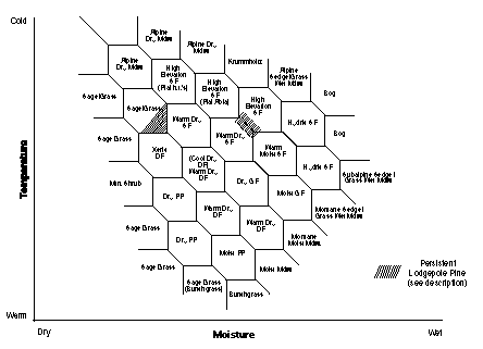
Because of the nature of the temperature and moisture interaction describing various habitat type classes, there is often a tendency to see overlap in the temperature and moisture relationships. For example, in figure 5 the range of temperature and moisture for Warm Dry Douglas Fire (DF) habitat type class is quite broad and is found in three areas while the range of temperature and moisture conditions for Dry GF (Grand Fir) is narrow and is even encompassed within the entire temperature and moisture range of the Warm Dry DF habitat type class. This overlap is of no surprise as one should expect to find all of these types of relationships because these habitat type classes are an artifact of a geographically continuous environment which varies over time and space. However, despite this reality, it is still widely supported that these habitat type relationships do hold true and represent for today the best and most current understanding about environmental gradients and habitat type class relationships.
What still remains to be identified is
what are all of the other environmental variables or dimensions
of the environmental gradient concept that need to be added in
order to define in multi-dimensional space the ability to predict
where each specific habitat type class can be found on the landscape.
For example, as we find through other existing or future research
that certain habitat type classes are also found on specific soil
types, parent material or some other variables within this environmental
gradient concept, these relationships can continue to provide
additional logic or reasoning for more precisely mapping habitat
type class relationships. However, in spite of the absence of
other supporting information to develop spatial habitat type class
relationships, the environmental gradient concept continues to
appear to be an appropriate methodology to begin to understand
where different habitat type classes occur and is for now the
method that is implemented within this modeling/mapping tool application.
In order to facilitate the environmental gradient mapping methodology within ArcInfo Grid, an interactive graphical user interface was written in ArcInfo aml. The interface allows the user to view and query geographic input layers, examine statistical relationships between collected field plot data and the input layers, develop spatial relationships for each habitat type class and run a grid function model that combines selected geographic input layers for each habitat type class to produce an output of predicted habitat type classes. The interface application, which has been named HABMOD see figure 6, also allows the user to view the modeled results, perform spatial queries, make specific edits to the output and produce a final output map.
Figure 6. HABMOD Interface Introductory Screen.
The user interface has been developed to incorporate both the best available field data and local expert knowledge for establishing spatial relationships for habitat type classes. In addition, the interface has also been designed to support an iterative modeling/mapping process. For example, once a user has defined the area they want to predict habitat type classes for, the next step is to identify the most appropriate geographic input layers for describing the environmental gradient and define the most appropriate values for predicting habitat type classes. Once selected input layers are identified and incorporated into the model computing environment, the user then needs to use the best available site based information or local expertise to develop logically structured spatial relationship queries for combining input layers to predict output habitat type classes. These queries are then submitted to the model interface, the model is run and an output of predicted habitat type classes is generated. This modeled output can then be displayed, queried and edited for a final map product or the user can go back to the spatial relationship queries, make spatial query adjustments and iteratively re-run the model interface until a final and/or acceptable modeled output is achieved. In other words, it supports an iterative modeling approach which can be refined by the user time and time again to produce a desire map output.
To accomplish this, the user interface is divided into 5 primary modules, the Input Layer Viewer, Field Plot Editor, Plot Statistics Generator, Model Equation Builder and the Model Output Viewer and Editor. Each of these modules support independent functions which contribute to the development and application of modeled and mapped output of habitat type classes.
The Layer Viewer Module allows the user
to display and query up to three input layers at a time, see figure
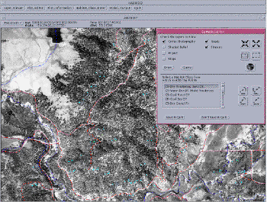
7. The Field Plot Editor module allows the user to add, delete
or move field plots of identified habitat type class sites for
use in statistical analysis and development of logically structured
relationships, see figure 8. The Plot Statistics Generator module
uses available habitat type class plot (i.e. point data) information
to generate statistics for each set of habitat type class plots
and all of the associated values with each identified input layer.
For example, a set of descriptive statistics is generated that
identifies values like the mean, the minimum, the maximum, the
standard deviation for each habitat type class and each input
layer. These descriptive statistics can then be used as a starting
point for developing the logical spatial relationships for predicting
each individual habitat type class. An example simplified logical
spatial relationship query to be entered into the model for predicting
a specific habitat type class might look like: Habitat Type Class
A = precipitation gradient > 56 and temperature gradient <
62 and slope > 15% and elevation > 4800 and elevation <
5600 and aspect = 7 and etc.
Figure 7. HABMOD Layer Viewer Module.
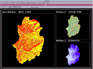
Figure 8. HABMOD Field Plot Editor Module.
Once all of the logical spatial relationship
queries have been established for each habitat type class, they
are then entered into the Model Equation Builder module and the
model is run. Once the model output has been generated, the results
can be displayed, queried and edited in the Model Output Viewer
and Editor. In this module, there is a set of querying and editing
tools that can be used to identify where there are potential problems
with the predicted output, the magnitude of the problems and whether
or not they can be simply edited or determine that a new model
run needs to occur.
APPLICATION OF ENVIRONMENTAL GRADIENT
MAPPING METHODOLOGY WITHIN THE INTERFACE FOR A PROTOTYPE AREA
In order to test the assumptions
of the environmental gradient mapping methodology described above,
a prototype test area was selected in west-central Idaho. The
selected test area was a 100,000 acre watershed known as the Gold
Fork watershed. As a large drainage, it is an ideal candidate
for testing the environmental gradient concept because the it
almost completely covers the range of environmental conditions
and habitat type classes that exist in west-central Idaho.
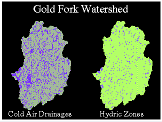
Using the best available expert knowledge of environmental gradients and habitat type class relationships and after a review of applicable and available geographic input layers, the base number of geographic input layers necessary to predict habitat type classes was reduced to six. The input layers used were ambient air temperature, solar radiation index, mean annual precipitation, topographic moisture, cold air drainage's and hydric zones see figures 9,10 and 11. Each of these input layers were selected and used in concert with the graphical environmental gradient tool in figure 5 to identify and define spatial relationships for predicting habitat type classes. For example, in using this methodology the ambient air temperature and solar radiation index input layers are used to characterize the temperature gradient axis in figure 5 while the geographic input layers describing mean annual precipitation and topographic moisture were used to characterize the moisture gradient axis. The other two input layers, cold air drainage's and hydric zones in figure 11, were used to separate out environmental affects that override other environmental gradient factors and result in cold air or hydric driven habitat type classes.
Figure 9. Examples of Model Input Layers for Describing the Temperature Axis of the Environmental Gradient Methodology.
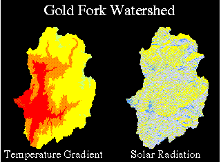
Figure 10. Examples of Model Input Layers
for Describing the Moisture Axis of the Environmental Gradient
Methodology.
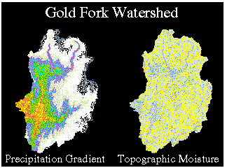
Figure 11. Examples of Other Model Input Layers that Influence Habitat Type Class Relationships in the Gold Fork Watershed.
Using each of these geographic input layers
and the spatial arrangement and alignment of habitat type classes
displayed in figure 5, logically structured spatial relationships
were established by identifying specific values from each input
layer to represent where along the temperature and moisture gradients
different habitat type classes occurred. These spatial relationships
were then entered into HABMOD, the user interface, and
an output grid was created combining all of the spatial relationships
for each habitat type class into an output layer of predicted
habitat type classes. This output layer was then displayed, queried
and iteratively re-run until an acceptable map of predicted habitat
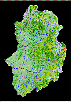
type classes for the Gold Fork watershed was created. Figure
12 illustrates an example of output that was created from this
habitat type class mapping and prediction effort. The generated
output of habitat type classes was then verified and validated
through a visual comparison to polygons of mapped habitat type
classes and to some extent with individually sampled and collected
field plot data. In addition, other accuracy assessment protocols
that reflect the integrity of the concept of the environmental
gradient has been identified and will be tested over the coming
field seasons.
While most of this methodology for predicting
and mapping habitat type classes is in no way complete, the ArcInfo
interface, HABMOD and the environmental gradient modeling concept,
used for predicting habitat type classes in west-central Idaho
does demonstrate great promise for continuing to understand and
predict habitat type class relationships on the landscape. It
also represents a tool that can be used to produce geographic
information that will support the implementation of ecological
land classification system to further support ecosystem management
objectives at the landscape level until other information sources
become available.
Figure 12. Predicted Habitat Type Classes for the Gold Fork Watershed
Using the Environmental Gradient Methodology.
LITERATURE CITED
Daubenmire, R. F. 1968. Plant communities:
a textbook of plant synecology. Harper and Row, N.Y. 300 pp.
Haufler, J. B. 1994. An ecological framework
for forest planning for forest health. J. Sustain. Forestry 2:307-316.
Steele, R., R. D. Pfister, R. A. Ryker,
and J. A. Kittams. 1981. Forest habitat types of central Idaho.
USDA Forest Service. Gen. Tech. Rep. INT-114. 138 pp.
AUTHOR
Stephen P. Warren
GIS Programmer/Analyst
Idaho Ecosystem Management Project
Boise Cascade Corporation
P.O. Box 50
Boise, Idaho 83728
(208) 793-2480
(208) 793-2712
email: steve_warren@bc.com