Using hydrologic modeling capabilities within the ArcInfo Grid module, we have developed a methodology for the monitoring and assessment of acid mine drainage on the surface waters of West Virginia. We map potentially affected areas from surface mining runoff to determine sampling locations, define and rank sub-watersheds based on their loading contribution, and use water quality data to estimate acid concentrations and loadings throughout a watershed. Proposed reclamation sites are identified and the effect on downstream conditions is modeled to show potential improvements. The input data requirements include Digital Elevation Models (DEMs), stream hydrology, precipitation, mined areas, and water quality data.
 

    The most common environmental problem associated with coal mining in West Virginia is acid mine drainage (AMD). AMD is defined as mine-water runoff with high concentrations of acidity, iron, manganese, aluminum, and suspended solids toxic to aquatic life (Squillace and Dotter, 1990). It is caused when coal seams are mined or opened during road construction and exposed to oxygen. AMD can enter streams as runoff from a point source (mine seep) or a non-point source (abandoned mine land). Less than five percent of active West Virginia mining operations have any water quality problems. The problems occur from abandoned mines, where operators have gone bankrupt releasing their responsibility to treat the pollution. The West Virginia Water Quality Status Assessment (WVDNR-OWR, 1996) found AMD to be the top water quality problem in the state polluting up to 477 streams totaling 2,427 miles.

    The West Virginia Division of Environmental Protection (WVDEP) Office of Mining and Reclamation approaches the AMD problem at the watershed level where physical interactions between pollution sources, the water chemistry, and land characteristics can be modeled to develop an appropriate treatment plan. Recognizing watershed characterization for AMD reclamation as a spatial problem, the WVDEP is using Geographic Information Systems (GIS) to store, retrieve, and analyze mining data for watershed characterization.

    To aid WVDEP in their reclamation decisions we have developed a methodology for modeling AMD in West Virginia. The methodology is built upon many of the hydrologic modeling capabilities of the ArcInfo Grid module to analyze surface runoff patterns and overland flow from hydrologic corrected DEMs. The following section discusses the objectives for characterizing the Lower Cheat River Watershed in West Virginia for AMD reclamation.

 Objectives

    Our main goal was to provide information to make better decisions in addressing the acid mine drainage problems for the Lower Cheat River Watershed. With a limited budget for AMD reclamation of abandoned mine lands, the WVDEP must efficiently address and progress through projects. Some of the questions we wanted to address included:

Where to focus water quality sampling?
What are normal flow conditions over different times of the year in the watershe?
Where are the most severely affected streams?
Which sub-watersheds or tributaries contribute the most to loading of the main stem Cheat River?
What effect would treatment have on downstream water quality?

    The first phase was to track the surface runoff from potential pollution sources across the landscape. By identifying the flow direction of potential sources of AMD, we could identify where in the stream runoff would enter. This information could then be used by the WVDEP to target areas for field sampling of the water quality.

    The second phase was to make flow estimates for all streams in the watershed. Knowing the average flow conditions for different months of the year allows for the calculation of pollution loadings. The modeling of flow also aids in designing reclamation structures to effectively handle the loads.

    The third phase was to use water quality data from the sampling sites, recommended in phase one, to model in-stream concentrations throughout the watershed. The assumptions of this modeling technique are described later in this paper.

    In the fourth phase we would delineate the sub-watersheds for all pollution contributing tributaries and rank the areas based on the loading to the main stem of the Cheat River. This regional analysis helps identify the locations of greatest concern in the watershed. It also gives an ordinal ranking of the watersheds for the amount of acid producing material to the main stem of the river. As a ranking tool it guides where to start reclamation work in the watershed.

    Using the results of the watershed ranking, phase five chooses a high-ranking sub-watershed and then analyzes the effects of treatment. We can demonstrate potential treatment sites and water quality improvements possible downstream.
 

Study Area

    The Cheat River Watershed covers approximately 1,400 square miles located in North Central West Virginia and a small part of Pennsylvania (Figure 1). The lower section of the watershed was chosen for this study because of the majority of mining and water quality problems in the basin occur in this region. Like many of the watersheds in the Appalachians, steep slopes dominate the landscape (Figure 2). Many of the tributaries of the Cheat River have been heavily impacted by mining activities for over 50 years (Figure 3). The River flows north from Rowlesburg to Cheat Lake, which has been dammed for flood control. The Cheat River Watershed has attracted much attention due to its national seventh ranking in a list of top ten endangered and threatened rivers and streams in the United States by the American Rivers, Incorporated. This national recognition increased public awareness of the condition of the Cheat River and prompted the need for a thorough inventory and evaluation of AMD sources and their subsequent impacts. Federal, state and local entities share concerns for the quality of the river because of its proximity to major population centers, recreational opportunities, and scenic beauty. The Cheat River provides some of the better white water rafting in the east when spring rains and snow runoff provide excellent recreational opportunities for boaters rafting the class IV rapids in the canyon (Figure 4).
 

 Data Preparation

    The input data used in our analysis consisted of 30m DEMs, 1:24k hydrology, monthly 30-year average precipitation grids at 90m resolution, and historical streamflow for USGS gauging stations. Before starting, much background work was required to prepare the data for hydrologic modeling in the Grid module of ArcInfo. We needed to create a hydrologicly correct DEM and a runoff grid. We have incorporated many of the techniques described by Saunders and Maidment (1996), Reed and Maidment (1995), Oliver et al. (1996). The following sections describe these steps in detail.

    The first step was in working with the DEMs. We downloaded and merged all DEMs for the study area to create a complete mosaic. The mosaicked DEM was then resampled from 30m to 10m to match the resolution of the rasterized stream network soon to be created. The Grid Fill command was then run to remove all sinks from the DEM.

    The second step involved working with the 1:24k-stream coverage. All rivers which were originally digitized with left and right banks were bisected with a single arc and tributaries connected. Next, all lakes, which resulted from inflowing rivers and streams (Figure 5), were bisected with a single arc (Figure 6). Any braided, stray or unconnected streams, ponds or lakes were removed from the study area coverage. The goal is to make sure water flow is represented with a single arc for the surface flow direction and flow accumulation Grid functions. When all streams were hydrologicly "corrected," the coverage was then converted to a grid with a resolution of 10m. The rasterized stream network was then thinned to ensure single cell stream width.

    The third step applies a "burn in" process by merging the raster stream network with the off-stream DEM cells raised 50 meters. It is important to keep the original DEM values for the stream grid so flow direction within the stream can be calculated. After the streams have been "burned" into the DEM, the DEM is then filled again and flow direction and flow accumulation grids calculated.

    We now have a hydrologicly corrected DEM with flow direction and flow accumulation grids. The fourth and last step is to create a runoff grid built on the relationship between precipitation and stream flow. We create a runoff grid by developing a statistical relationship between historical stream flow and 30 year average annual precipitation grids. The precipitation grids are 90m in cell size and have been extrapolated to grid format from the observation collection points. The historical stream flow is recorded for the same time that the precipitation grids were recorded 1963 to 1993. For each gauging station we delineate the watershed for that location and then find the average precipitation for the watershed area. We then convert the flow in cfs to a measure of volume in m³/year. The next step is to divide the flow volume (now in m³/year) by the watershed drainage area in m² to calculate an equivalent depth of recorded streamflow in mm/year. We then regress the value of the equivalent depth of recorded stream flow versus the average annual precipitation to find a regression equation to apply to the precipitation grid to estimate runoff (Saunders and Maidment, 1996). The runoff grid is used to represent the relationship between how precipitation relates to stream flow. We also calculate a cumulative runoff grid by running a weighted flow accumulation with the runoff grid itself. It is used in the modeling of instream concentrations along with flow estimation. The runoff grids are used with flow accumulation and flow direction grids to model the flow estimation, pollutant concentrations and potential maximum yearly loadings. We will cover these topics in the next sections.

Phase 1 - Identifying potentially affected streams

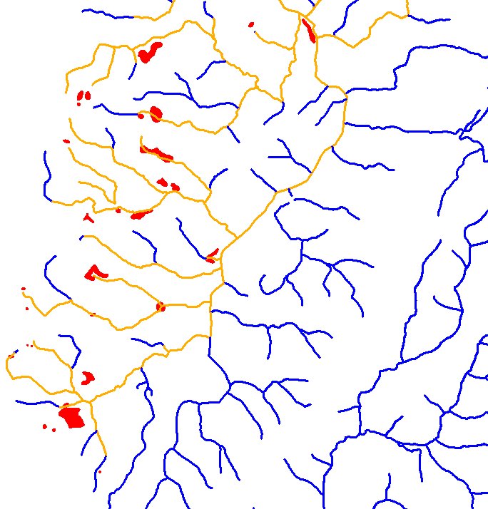
    After preparing the data for hydrologic modeling, we could then start proceeding through each of the phases to characterize the watersheds for AMD reclamation. The first phase was to track the surface runoff from potential pollution sources across the landscape. The sources for AMD may come from abandoned mine lands, bond forfeiture sites, and coal refuse piles. We assumed that each is a pollution source and a contributor to acid mine drainage runoff during a precipitation event. Our goal was to find all the streams and where in the streams the runoff from these sites would cause problems. This information would help determine which streams to sample.

    We first digitized all abandoned mine lands, bond forfeiture sites and coal refuse piles from field inspection quads and converted them to grids where they were combined to create one grid of all the potential pollution sources. A value of 100 was assigned to each of the pollution source cells and then used as the weight grid in the flow accumulation function. The final vector stream coverage contained an item called "grid-code" which indicated the presence of runoff from the pollution sources (Figure 7).

Phase 2 - Estimate Flow

    In watershed characterization, it is important to determine loadings in lb/day or Tons/year for the amount of acid load polluting a stream. Being able to estimate stream flow for all streams in the watershed provides scenarios in which to simulate different conditions that may occur during the year. For example, by estimating and modeling the likely high, low and average flow conditions on a monthly basis, reclamation strategies and systems can be more effectively built to match the conditions that would occur over the year.

    To calculated stream flow in cubic feet per second we used the runoff grid as the weight grid to create a cumulative runoff grid, which is in meters³ per year. We then multiplied it by the number of cubic feet per cubic meter and divided by the number of seconds per year. When converted back to vector format the stream coverage will have the flow in cubic feet per second as the grid-code item (Figure 8).

 Phase 3 - Model stream acidity

    The third phase for characterizing watersheds for acid mine drainage problems is to model the in-stream acidity. We can also model the iron, manganese and sulfur concentrations with the method we will describe for acidity. Stream acidity is modeling assuming that the streams have the same hydro-geometric properties (stream slope, roughness, width and depth), and that the streams have the same ecological rate constants (re-aeration rates, pollution decay rates and sediment oxygen demand rate). The concentrations modeled can be thought of as the maximum potential concentrations with the available data and under the stated assumptions (Saunders and Maidment, 1996).

    We model acidity by first identifying all sampling locations that have a recorded acidity level. We then use these points, which may be in-stream samples or off the stream from a mine seep, and delineate sub-watersheds for their locations. The sub-watersheds are then assigned the value of the acidity from the sampling point. Essentially we then have areas which are known to contribute the amount of acidity defined by the sampling location. The defined areas indicate measured acidity concentrations. Multiplying these areas by the runoff grid creates a cell based loading grid. The cell based loading grid is used as the weight grid in the flow accumulation function. The resulting grid will provide the in-stream acidity concentrations for all cell locations. When converted back to vector format, the streams indicate concentrations in the grid-code item. This technique allows the streams to show the combination of pollutants to stream water quality from point and non-point sources over the landscape (Figure 9).

 Phase 4 - Sub-watershed Acid Load Analysis and Ranking

    With the modeled stream acidity and estimated flow, we can now calculate the acid load from each stream into the mainstem of the Cheat River. The loading should be thought of as the potential maximum because of the assumptions mentioned earlier. We delineate sub-watersheds for the mouths of tributaries where sampling data was collected. Displaying sub-watersheds in a region ranked by acid load provides a visual recognition of problem areas and acid load contribution to the Cheat River mainstem (Figure 10). It can lead researchers to target the most severely impacted watersheds most efficiently. While this watershed ranking is only based on acid load, other sub-watershed level characteristics can be included to further define the rankings. For example the benefits from reclamation could be compared and ranked across the sub-watersheds to better select and identify where to work. For more information, see Strager et al. (1995), who combined additional evaluation criteria and the preferences of various stakeholders to rank watersheds affected by AMD.

 Phase 5 - Select Treatment Sites and Model Water Quality Improvements

    Using the results of phase four, the sub-watersheds contributing the most acid load to the mainstem Cheat River can be identified. By selecting one of the sub-watersheds from the list, we then proceed in phase five to test different treatment scenarios for AMD reclamation (Figure 11). The scenarios we test include finding how much acid reduction is needed and what effect will remediation strategies have on the AMD problem. We can find where to treat by querying any stream location for the amount of acid load present. We test remediation strategies by digitizing in the location of a constructed wetland or a limestone channel and attributing it with the amount of acid reduction we would expect the system to generate to treat the stream acidity (Figure 12). The digitized remediation strategy is then used as a weighted grid in the flow accumulation function to test the effects of treatment. The location and expected acid reduction can all be altered to find the scenario which would work best. This provides valuable information to the reclamation specialist working toward a reclamation plan.
 

    The main advantage of the methodology discussed is in providing information to make better decisions for addressing the AMD problems in West Virginia. We have presented a framework to help guide where to sample water quality, estimate flow from runoff grids, calculate the transport of pollutant concentrations in streams, delineate and rank sub-watersheds based on loadings to the mainstem, and provide the ability to test treatment scenarios for downstream water quality improvements.

    The hydrologic modeling tools available in ArcInfo Grid provided the ability to extract the topographic structure from the digital elevation data for characterizing the Lower Cheat River Watershed for its AMD pollution sources. By using a hydrologicly corrected DEM from preprocessing work we are able to improve the accuracy of runoff directions, watershed delineations, and the transport of pollutants within the streams.

    Future directions of this work include creating an application and interface in ArcView as a loadable extension which would guide the user through each of the phases discussed in this paper. The Spatial Analyst for Arcview contains many of the key ArcInfo Grid functions for watershed delineation, flow direction and flow accumulation that would be needed. We also plan to improve the estimation of the runoff grid by combining other landscape-based variables to improve its accuracy. Other areas of research in which we are currently using the methodology include Total Maximum Daily Load Analysis in West Virginia, and poultry litter and phosphorus loading in the Potomac River Watershed, West Virginia.

    I would like to acknowledge the work at the Center for Research in Water Resources at the University of Texas at Austin (http://www.ce.utexas.edu/prof/maidment/gishydro/home.html) specifically Dr. Maidment and his graduate students for the wealth of information presented on their website for hydrologic modeling using GIS.

    I would also like to thank Bill Saunders from the Texas Natural Resource Conservation Commission for his helpful comments and direction in this work.
 
 

Esri 1992. A Cell Based Modeling with Grid 7.0: Supplement - Hydrologic and DistanceBased Modeling Tools. Environmental Systems Research Institute, Redlands, California, USA.

Olivera, F., R. J. Chareneau and D. R. Maidment. 1996. CRWR Online Report 96-4: Spatially Distributed Modeling of Storm Runoff and Non-Point Source Pollution Using GIS.

Reed, S.M., and D.R. Maidment. 1995. CRWR Online Report 95-3: A GIS Procedure for Merging NEXRAD Precipitation Data and Digital Elevation Models to Determine Rainfall-Runoff Modeling Parameters.

Saunders, W. K. and D. R. Maidment. 1996. CRWR Online Report 96-1: A GIS Assessment of Nonpoint Source Pollution in the San Antonio Nueces Coastal Basin.

Strager M. P., Fletcher J. J., Phipps T. T. and C. B. Yuill. A Compromise Programming Model to Select Acid Mine Drainage Affected Watersheds for Reclamation. Journal of Soil and Water Conservation, forthcoming.

Squillace, M., and E. Dotter. 1990. The Strip Mining Handbook. Environmental Policy Institute and Friends of the Earth: Washington, D.C.

West Virginia Department of Natural Resources Office of Water Resources. The West Virginia Water Quality Status Assessment 1996. Charleston, West Virginia.

 
Author Information

Michael P. Strager
Research Assistant
Natural Resource Analysis Center
Division of Resource Management
West Virginia University
Morgantown, WV 26506-6108
Telephone: 304-293-4832 ext. 4453
Fax: 304-293-3752
Email: mps@wvu.edu

Jerald J. Fletcher
Professor
Division of Resource Management
West Virginia University
Morgantown, WV 26506-6108
Telephone: 304-293-4832 ext. 4452
Fax: 304-293-3752
Email: jfletch@wvu.edu

Charles B. Yuill
Associate Professor
Division of Resource Management
West Virginia University
Morgantown, WV 26506-6108
Telephone: 304-293-4832 ext. 4451
Fax: 304-293-3752
Email: charlie@caf.wvu.edu