Habitats and ecotopes in the coastal zone
Abstract
In order to predict the effects of proposed measurements on (aquatic)
ecosystems the use of habitats and ecotopes has risen as a new tool in
the last decade. In this paper working specifications of both terms are
given. At present in the Netherlands, a method has been developed to
distinguish ecotopes and habitats for the marine and estuarine systems
using a multitier concept. This concept is based on the relations
between species, communities or ecosystems and different abiotic
parameters, if necessary completed with human use/management. The
relations are determined and processed into maps per parameter (single
tier maps or monoparametric Habitat and Ecotope Maps). These maps are
merged into (multiparametric) Ecotope and Habitat Maps (multitier
maps).
This procedure is carried out in a GIS (Geographical Information System),
using the Gridmodule in UNIX ArcInfo, with a user-friendly application
written in AML. The ample use of form menus provides also non-GIS-
specialists a GIS toolbox that can be used very easily. Due to the
multitier concept it is easy to add new information, i.e. a new,
proposed situation computed with a computermodel. It is also possible
to examine the state of the art about the relationships between parameters
and species/communities, using both statistical and intuitive
knowledge. In fact, the application can be seen as a spatial model,
possibly as part of a larger Decision Support System.
1. INTRODUCTION
Policy makers and researchers often want to know the effects of
proposed measurements on aquatic ecosystems on different levels (single
species, communities or the entire ecosystem). One way to investigate
this is the use of HABITATS and ECOTOPES. It is a problem that these
terms are defined ambiguously. This leads to ample discussions
that distract the attention from the actual applicability of the
concept of ecotopes and habitats as a way to condense ecological
information for management purposes and policy-analysis. Therefore, in
this paper, "working specifications" of both concepts are given (see 2),
particularly aimed at their practical use.
Using these working specifications, a method is being developed to
distinguish ecotopes and habitats in the marine and estuarine systems
in the Netherlands using a multitier concept, the HABIMAP-concept. This
concept is based on the relations between species or communities and
different abiotic parameters, when necessary completed with information
on human use and management.
This paper describes the general concept of this multitier approach to
obtain Habitat and Ecotope Maps (see 3) and the way in which this is
being worked out in GIS (see 4). Some possible ways to use the concept
are highlighted in 5.
We apologize for the poor quality of the maps
linked to the document. The only way to produce proper jpg-files of
our GIS-maps was scanning the hardcopy output and process them into
this format.
2. HABITATS AND ECOTOPES, SPECIFICATIONS
Ample discussions are being held on the definitions of ecotopes and
habitats and many other terms in this respect. A problem is that both
terms are defined ambiguously. Both terms are used as synonyms as
well as different terms and, moreover, they are often mixed up. Many
terms are added to increase the confusion. In order not to be
trapped into these discussions, we have made working specifications for
both terms, aimed at their practical use for research and management,
which are given below.
A HABITAT is the environment of one species defined by a combination of
several abiotic parameters, if necessary, supplemented with human
influences. One species may need multiple habitats in multiple
areas; i.e. a wading bird may need a breeding habitat in the arctic
tundra, a feeding habitat along the migratory routes in NW-Europe and a
feeding habitat in the hibernation area in NW-Africa. Meanwhile a lugworm
may need two types of sandy substrate in the intertidal zone in the
same estuarine system, but higher in the intertidal zone for the
juveniles and lower down for the adults.
Habitats are defined by the individual relations between a species and
the determining abiotic parameters, like soil composition, current
velocity, waves, geomorphology and depth. The result is a Habitat Map
which generally covers only a part of an area. Generally the
relations between a species and the determining parameters can be
expressed in some sort of an optimum curve. The Habitat Map indicates
the living conditions for the species involved on a scale of 0-100%.
An ECOTOPE is the environment of a community and is defined similarly
as habitats by a combination of several abiotic parameters. The result
is a map with one or more ecotopes, which can cover the whole area,
depending on the number of communities involved. The communities to be
distinguished may be, for example, the community of soft sediment infauna
in the intertidal area (e.g. the lugworm-community) or the community of
subtidal rocky shores (e.g. the community of brown algae).
However, it is also possible to define "ecotopes" as sensitive to certain
human activities like oil spills or bottom trawl-fishery. This type of
ecotopes is determined depending on questions arising in management and
policy-making. This way an Ecotope Map can be considered to be a "map
in which the ecological relevant information, related to a specified
management question, has been assembled".
3. THE HABIMAP-CONCEPT, A MULTITIER CONCEPT
3.1 General introduction
The
multitier HABIMAP concept
is based on the
following general assumption. The presence of a species or a community
is determined primarily by a combination of a number of abiotic
parameters, soil composition, depth, wave action and climate, and
may be influenced secondarily by human activities such as fisheries,
recreation and shipping.
Relations can be determined between species/communities and these
parameters, i.e. a range for each parameter in which each
species/community may be present. These relations can be combined with
the single parameters. As the parameters generally can be presented in
some sort of maps, these relations can be expressed into "maps with
possible occurrence" per parameter (single tier maps or monoparametric
Habitat/Ecotope Maps). These single tier maps are combined subsequently
into Habitat and Ecotope Maps (multitier maps or multiparametric
Habitat/Ecotope Maps).
3.2 Preparations to make the maps
3.2.1 The data
The procedure is underlain by the abiotic data in the form of
monoparametric maps such as depth, soil composition,
wave action, (maximum) current velocity and geomorphology.
Water quality parameters like salt
or nutrients are
also possible data. Some of these parameters are mapped in an integral
way (like geomorphology), others are based on the interpolation of a
number of sample points (e.g. water quality, depth, soil composition)
and some are the result of model calculations (such as current velocity
and wave action). When possible a continuous map legend is preferable
to apply; as this offers the best opportunity to make combinations with
the relation curve/table. However, in some cases (like geomorphology)
only discontinuous legends are available. All maps are, if still
necessary, converted into grid maps, as the calculations are all done
on a grid basis.
With respect to the choice of the parameters, a couple of things have to
be kept in mind. When using interpolation techniques, it is very
important that the final result resembles the reality as well as possible.
This implies that quite often it is not possible to use a simple linear
interpolation technique, but that more sophisticated techniques are
required which take additional information into account (or that the
interpolation is done "by hand" by a specialist).
For some parameters a conversion into a derived parameter is important.
As an example; in an intertidal area the absolute height of the surface is
not the important factor, but rather the period of exposure or immersion.
The derived combination of surface height and tidal range yields a workable
parameter. For other parameters this can be necessary as well. For
instance during wave action, the orbital velocity at the bottom may be
used as the relevant parameter.
When using results from a computer model, it is important to give due
consideration to the input conditions for the model, as well as the
desired results. e.g. for a wave action model one should choose a storm
condition with a relative high frequency of occurrence (e.g. 1x/year)
for relative short-living species, and with a lower frequency of
occurrence (e.g. 1x/5 year) for longer-living species.
Sometimes it is important to take seasonally (climatic) aspects into
account. In an estuary there might be seasonal determined differences
in river discharge leading to seasonal changes in water salinity. In
this respect, changes in air temperature or water temperature also have
to be mentioned.
3.2.2 The relations
For every species or community involved, a relation with each
determining parameter has to be specified, i.e. the parameter
boundaries, between which, the species or community may be present for
that particular parameter. These relations may be determined by
research or obtained in a more empirical way or even may be based on
intuition. Depending on the type of data and the type of legend used
(continuous or discontinuous), the relation may be expressed as an
optimum curve
, an
S-shaped curve
or in discrete steps.
In the HABIMAP-concept for Habitat Maps (single species) optimum curves
are used. This results in "living conditions" on a scale of 0-100% (no
living conditions and maximum living conditions resp.). For the Ecotope
Maps (communities) discrete steps are used, resulting in a community
being either present or absent.
3.3 Composing Habitat Maps
3.3.1 Monoparametric Habitat Maps
The first step in composing a Habitat Map is the creation of a number
of monoparametric Habitat Maps for the parameters relevant for that
species. This is only a matter of substitution. Each cell value of the
grid in the abiotic map is compared with the relation curve or table
and is substituted by the corresponding value. If necessary, grid values
are interpolated between the adjoining table values.
The units are percentages (0-100%), indicating the living conditions in
each grid cell for that parameter; 0% indicates no living conditions
and 100% maximum living conditions. Using the monoparametric maps and
the determined relations, an example is given for the
relation Cockle - height
and
the relation Cockle - chloride.
3.3.2 Multiparametric Habitat Maps
The final Habitat Map is made by combining a number of monoparametric
Habitat Maps into one,
multiparametric Habitat Map.
The method used to combine these monoparametric Habitat Maps
influences the outcome. Some possibilities are indicated here:
A first method is a straight forward multiplication of the single
Habitat Maps: the percentages of each grid cell are multiplied by
each other as decimals and then multiplied with 100. Some examples:
1) if in any monoparametric map a grid cell has the input value 0 the
output value will also be 0;
2) if all input values are 100% the output value is also 100%;
3) when for three maps the input values in a specific grid cell are
50%, 50% and 100%, the output value after multiplication will be 0.5 *
0.5 * 1.0 *100% = 25%.
4) the grid cell input values 50%, 50% and 50% result in an output
value of 0.5 * 0.5 * 0.5 * 100% = 12.5%.
5) the grid cell input values 100 x 100 x 12.5 also give 12.5%.
With this method, no difference is made between a series of input values
with all medium high values (Ex. 4) and a series with some high and one
low value (Ex. 5). Even a combination of rather high values may
result in a rather low output value (Ex. 3). Some sort of (log, square
root) transformation may give some optical improvements in stretching
the lower part of the scale in benefit of the upper part, but it does
not improve the problem of the dissimilarity between equal values as is
the case in Ex. 4 and Ex. 5.
A second method is that the parameter with the lowest grid cell input
value determines the final result: the lowest grid cell input value of
any monoparametric Habitat Map will become the output value for that
cell in the multiparametric Habitat Map. This means that in Ex.1 and
Ex. 2 the output value does not change (0% and 100% resp.), but that in
Ex. 3 and Ex. 4 the output value will become 50% and in Ex. 5
12.5%.
A third possibility is to attach a degree of importance to each
parameter. In this way, some parameters can be considered as more
important than others (which quite often is the case). All in all, it is
clear that the method of combination is a point that must be considered
carefully.
3.4 Making Ecotope Maps
An Ecotope Map is produced in a similar way as a Habitat Map. However,
now each parameter used is classified in discrete steps, legend
classes, instead of the optimum curves as are used for the Habitat
Maps. E.g. a classification of the
parameter 'height'.
can be: < MSL-10m (channels), MSL-10m - MSL-5m
(gullies), MSL-5m to MLW (shallow water) and MLW to MHW (intertidal),
and a classification of the
parameter 'emersion time'.
can be: 0% - 50%
emersion time (low littoral), 50% - 85% emersion time (middle littoral), 85% - 95% emersion time
(high littoral) and 95% - 99% emersion time (salt marsh etc.).
A classification of the
parameter 'current velocity' .
can be: current velocity >
1 m/sec (high dynamic), current velocity 1 - 0.5 m/sec (dynamic), current velocity <
0.5 m/sec (low dynamic),
and a classification of the
parameter 'orbital velocity' .
can be: orbital velocity > 0.4 m/sec (high dynamic),
orbital velocity 0.4 - 0.2 m/sec (dynamic), orbital velocity < 0.2 m/sec (low dynamic).
In combination the last two parameters can also be one group parameter,
hydrodynamics .
which can be classified as: current velocity >
1 m/sec or orbital velocity > 0.4 m/sec (high dynamic), current velocity
1 - 0.5 m/sec or orbital velocity 0.4 - 0.2 m/sec (dynamic), current velocity <
0.5 m/sec or orbital velocity < 0.2 m/sec (low dynamic).
For all relevant abiotic parameters such a classification has been made. The
grid cells in the monoparametric maps are compared with the
classification tables and the cells get the corresponding
classification value. In order to make the Ecotope Map these
monoparametric maps are combined via a direct overlay technique. In
this case the output values are discrete values instead of percentages
as used in the Habitat Maps. Finally, all areas concerned will get a
label based on the combined classifications. Using the three parameters
mentioned above, some ecotope classes may be: the "subtidal dynamic"
ecotope or the "low intertidal, low dynamic" ecotope.
It is also possible to add specific species or communities to this classification,
e.g. musselbeds or seagrass fields. It is essential that the species/communities
are actually mapable. This means that only species that are detectable on the
surface can be used, preferable by aerial photographs or something similar.
In this way a general ecotope map can be made.
Besides more specific ecotope maps can be made, oriented to a specific species
or community; e.g. an ecotope map of benthic animals ,
an ecotope map of wader birds or an
ecotope map of fish .
In ecotope maps like these such classification boundaries are chosen which are
relevant for the groups concerned. In 5 some more possibilities are presented.
3.5 Scenario maps
Besides parameter maps with the actual situation, maps of new
situations can be used as well. Historical maps can be used to
investigate the historical situation, and determine a
"historical reference" situation. Moreover, parameter maps indicating
new situations, scenario maps, can be used to investigate possible
consequences of certain management measurements or new activities (see
also 5).
4. THE STRUCTURE OF THE APPLICATION "HABIMAP"
4.1 General outline
The application HABIMAP is an ArcInfo application using the GRID-,
ARCEDIT- and ARCPLOT-module. The application is menu-guided and the
menu interfaces are designed to be user-friendly to researchers and
policymakers without much knowledge of GIS or ArcInfo. The user
interface and functionality are designed using AML and FORMMENUS. The
application is using an internal database (an INFO-database).
4.2 The database
The
database
is organised in six subsequent
levels:
1. The theme
The theme of a dataset is often divided into two aspects: theme and
subtheme. For example: the theme of a depth map is: physics, subtheme:
depth. The theme of the soil map is also physics, subtheme: grainsize.
The theme of the chloride map is: water quality, subtheme: salt. The
FIRST directory layer in the database contains the themes, the SECOND
layer contains the subthemes.
2. The co-ordinate system
The Dutch coastal zone is relatively small, enabling the use of one
grid, the New Dutch Topographical Grid. However the data of the North Sea
are stored in the UTM31 system. The THIRD directory layer distinguishes
between these co-ordinate systems.
3. The region
The Dutch coastal zone is divided into regions on three areal scale
levels: "main region" (e.g. Western Scheldt), "middle region" (e.g.
Western part of the Western Scheldt) and "detail region" (e.g. one
sandflat). The level on which a dataset is stored depends on the type
of data involved: a depth map or a soil map is stored in the "main
region" level, a vegetation map is stored in the "detail region" level.
The FORTH directory layer therefore contains the "main region" level,
the FIFTH layer (if present) the "middle region" level and the SIXTH
layer (if present) the "detail region" level.
About the name conventions on the directory level: both the theme and
the subtheme directory name consists of four characters and each region
directory level is named with six characters. The name of a particular
dataset consists of the region name (six char.), the year of survey
((still) two char.) and extensions (like .cov or .grid or .inf) if
necessary. The theme name is not included in the file name.
4.3 The user interface
The application is organised per region. First the region level is
chosen: "main region", "middle region" or "detail region". This will be
the workspace in this HABIMAP session where the user data are stored.
After the region selection the MAIN MENU appears.
In the MAIN menu the button OPERATIONS opens the menu OPERATIONS and
from there on the menu HABITAT MAPS can be selected. In this menu a
species is selected as well as the relevant abiotic parameters. Per
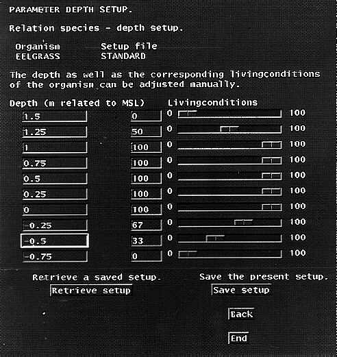
parameter, the button SET UP opens a
setup menu
in which the current
relation table between the selected species and that specific abiotic
parameter is described. The set-up menu offers the possibility to change
the values in the relation table. After all selections have been made,
the button CALCULATIONS starts the calculations for a Habitat Map
coverage.
Also, from the menu OPERATIONS, the menu ECOTOPE MAPS can be selected. In
this case no species are to be selected, but only abiotic parameters
and relation tables. The rest of the set-up is quite similar to that
of the Habitat Maps.
In the MAIN menu, the button PRESENTATION opens a series of menus to set
up a map. First the general map set-up is chosen. Some possibilities in
this respect are: one or four maps on a plot; with or without a
scalebar, with or without area calculations in the legend and output language. Next,
the geodatasets are chosen. Third, the paper size, printer, shade set, etc. are
selected. After the map has been drawn, there are possibilities to zoom in at
special subregions of interest and to add text to the map. The final map can be stored
(optional) as a plot file.
5. Use of Habitat Maps and Ecotope Maps
Habitats and ecotopes, as defined above, may be used in different ways in
research, Environmental Impact Assessment and management. Some
possibilities are highlighted here.
RESEARCH: For researchers a Habitat Map, made by the HABIMAP-concept,
offers a good possibility to visualise and test their knowledge on the
relations between an individual species and the determining abiotic
parameters, both per parameter separately and for a set of parameters.
Moreover, it is also possible to get indications on the importance of
the individual parameters for that species. Besides knowledge from
literature and experiments, it is also possible to test intuitive
knowledge, that is knowledge that is not quite formalised in figures
but that is only present "in the mind" of a researcher. Testing is done
by making a Habitat Map for a certain species and comparing it with the
actual distribution data of that species. In addition, it is possible to
make distribution maps of a species based on the determining physical
and chemical factors (instead of by interpolation of a couple sample
points).
Generally, it is easier to describe habitats for species living in/on
the substratum like soft-sediment fauna (mussel, lugworm, seagrass),
than it is for mobile species like birds and fishes. For the second
group generally their presence is primarily determined by the
availability of food. In such a case it might be possible to use the
presence of their staple food source (made as a Habitat Map) in
combination with availability of the food (period of emersion/immersion
or water depth) to obtain a Habitat Map. Besides, presently research results are
becoming available in which a direct relation has been made between wader birds
and several relevant abiotic parameters such as soil composition and
emersion time.
ENVIRONMENTAL IMPACT ASSESSMENT: Both Habitat Maps and Ecotope Maps,
made by the HABIMAP-concept, offer good possibilities to investigate
possible consequences of proposed management measures (e.g. bottom
trawling-fishery) or construction activities (e.g. channel dredging,
dam construction). For the policy analysis of a proposed construction
work, several scenarios are generally developed. With the help of
computer models or with "common sense", one can make new monoparametric
maps adapted to the possible scenarios. These "scenario maps" can be
used instead of the maps with the actual situation. The resulting
Habitat or Ecotope Maps per scenario can be compared with the actual
Habitat or Ecotope Maps and with each other in order to get insight in
the possible consequences of the scenarios. Moreover, GIS offers a good
possibility to compare these maps by "subtracting" them from each
other, making maps of changes.
MANAGEMENT: The re-introduction of an endangered species can be
tested beforehand with the help of a Habitat Map. This map will show
whether there are places with suitable living conditions in the area
for that species and if so, of what size and where. By using different
management scenarios (see above) one can investigate the effect of
possible measurements to improve the living conditions.
As ecotopes can also be discerned from a management point of view, it is
possible to investigate what areas are sensitive to bottom
trawling-fishery or oil spills in case of a disaster. In the latter
case, the classification of the depth parameter could be like this:
below MSL (no oil pollution), MSL to MHW (temporary pollution) and
above MHW (definitive pollution zone. Additionally the soil map may be
classified in: sand (oil easy to remove), muddy sand (oil hard to
remove) and muddy sand + mud (oil very difficult to remove). The
combination of the relevant monoparametric maps classified according to
this specific management question will lead to an "Ecotope Map"
indicating the sensitivity of areas to oilspills.
For use like this it is probably better to consider ecotope maps as
"Ecological Maps", being maps in which ecological information relevant
for a specific use is compiled. With respect to this purpose the application
might be coupled to a Decision Support System, like a spatial model.
ACKNOWLEDGMENTS
We wish to thank Mr J Perdon for his contribution in preparing the
figures, and Mrs G J Goedheer and Mr V. Hoyt for critical reviewing
the manuscript on usage of English.
Name: Johan F. Ruiter
Title: ING
Organisation: National Institute for Coastal and Marine Management
(RIKZ).
Mailing Address: POBox 207
City: Haren
Country: The Netherlands
Postal Code: NL 9750 AE
Telephone: 0031505331363
Fax: 0031505340772
E-Mail Adress: j.f.ruiter@rikz.rws.minvenw.nl
Name: Dick J. de Jong
Title: DRS
Organisation: National Institute for Coastal and Marine Management
(RIKZ).
Mailing Adress: POBox 8039
City: Middelburg
Country: The Netherlands
Postal Code: NL 4330 EA
Telephone: 0031118672284
Fax: 0031118616500
E-Mail Adress: d.j.djong@rikz.rws.minvenw.nl