1998 Esri User�s Conference
July 25-31, 1998
San Diego, California
HEC-PrePro v. 2.0: An ArcView Pre-Processor
for
HEC�s Hydrologic Modeling System
Francisco Olivera, Seann Reed and David Maidment
University of Texas at Austin - Center for Research in Water Resources
Austin, Texas
Abstract
HEC-PrePro v. 2.0 -- a system of ArcView scripts and
associated controls -- has been developed to extract hydrologic, topographic
and topologic information from digital spatial data of a hydrologic system,
and to prepare an input file for the Hydrologic Modeling System (HMS) developed
by the Hydrologic Engineering Center (HEC) of the United States Army Corps
of Engineers. Starting from the DEM and a SCS curve number grid, HEC-PrePro
v. 2.0 delineates streams and watersheds, calculates parameters
for each of them, determines their interconnectivity, and prepares an input
file for HMS that includes the computed hydrologic parameters. After running
HMS, hydrographs at any selected point in the river system can be obtained.
Using HEC-PrePro v. 2.0, the determination of physical parameters
for HMS is a simple and automatic process that accelerates the setting
up of a hydrologic model and leads to reproducible results.
Table of Contents
1. Introduction
HEC-PrePro v. 2.0 -- a system of ArcView scripts
and associated controls -- has been developed to extract hydrologic, topographic
and topologic information from digital spatial data of a hydrologic system,
and to prepare an input file for the Hydrologic Modeling System (HMS) developed
by the Hydrologic Engineering Center (HEC) of the United States Army Corps
of Engineers.
HMS is a computer program used to model rainfall-runoff processes in
a watershed or region, and is an improved Windows version of the well-known
HEC program HEC-1. One component of an HMS model is the basin file,
which stores hydrologic, topographic and topologic information for the
system. Based on data from GIS layers, HEC-PrePro v. 2.0 prepares
a basin file in ASCII format, which when opened by HMS automatically
creates a topologically correct schematic network of sub-basins and reaches,
and attributes each element with selected hydrologic parameters.
HMS is a very flexible program that allows the user to choose among
different loss rate, watershed routing (i.e., unit hydrograph), and baseflow
models for the sub-basins, as well as different routing methods for the
streams. However, because some of these models and methods depend on hydrologic
parameters that can not be extracted from readily available spatial data,
HEC-PrePro v. 2.0 does not estimate parameters for all methods
supported by HMS. At the moment, HEC-PrePro v. 2.0 is capable
of determining parameters required by the Soil Conservation Service (SCS)
curve number method for loss rate calculations, the SCS unit hydrograph
model for watershed routing, and either the Muskingum or lag method for
flow routing in the streams (depending on the reach length).
Using HEC-PrePro v. 2.0, the determination of physical parameters
for HMS is a simple and automatic process that accelerates the setting
up of a hydrologic model for HMS and leads to reproducible results.
2. Previous work
HEC-PrePro v. 2.0 is the synthesis of several GIS and
hydrologic modeling applications developed over the last years. In this
section, the existing GIS technology and HEC hydrologic modeling programs,
used in Hec-PrePro v. 2.0, are reviewed.
The raster-based GIS environment is very suitable for hydrologic modeling,
mainly because raster systems have been used for years, and a mature understanding
has been achieved and efficient and useful algorithms have been developed
for terrain analysis. Grid systems are ideal for modeling topographically
driven flow, because a characteristic of this type of flow is that flow
directions do not depend on any time dependent variables, say flow or water
depth. Consequently, raster GIS software includes hydrologic functions
as part of its capabilities, which allow one to determine flow direction
and drainage area from digital elevation models (DEM�s), and to delineate
stream networks and watersheds. DEM�s are available at different resolutions:
30 meters (USGS a), 3 arc-seconds (approximately 90 m) (USGS b), and 500
meters (USGS c) for the entire United States, and 30 arc-seconds (approximately
1 Km) (USGS d) for the whole earth.
Jensen and Domingue (1988) and Jensen (1991) outlined
a grid scheme to delineate watershed boundaries and stream networks. The
scheme uses digital elevation data to assign a flow direction from each
cell in a grid to one of its eight neighboring cells according to the path
of the steepest descent (i.e. each cell of the watershed is connected to
the lowest of its neighbor cells). The cells contributing flow to the pour
point can be counted, representing area, and the cells having no contributing
flow define drainage boundaries. Cells having a flow accumulation in excess
of a threshold value are classified as stream network cells.
Functions to delineate streams and watersheds that use the Jensen and
Domingue algorithms are available through Avenue requests in ArcView 3.0a
Spatial Analyst 1.1. The Hydrologic Modeling ArcView extension, distributed
by Esri with the Spatial Analyst , makes this functionality accessible
to users who are not familiar with Avenue. A more specialized set of procedures
that allows the user to interactively delineate watersheds is available
through the Watershed Delineator ArcView extension. The Watershed Delineator
was developed by the Applications Programming group at Esri for the Texas
Natural Resources Conservation Commission (TNRCC). The Watershed Delineator
pre-processes the terrain data, and delineates watersheds to any point,
line segment, or polygon selected interactively by the user from the map.
Pre-processing includes defining flow directions and drainage areas for
each cell, and defining a sub-watershed base map at a specified drainage
area threshold. Using pre-processed data, when the end user makes a delineation
at a point, only those DEM cells within the base sub-watershed containing
the selected point need to be processed, even if the selected pour-point
is on the main river and many sub-watersheds are upstream of it. To provide
this functionality, the drainage sequence of sub-watersheds in the base
map is determined within the vector domain. The Spatial Analyst functionality
to make raster-to-vector conversions (to convert strings of cells into
lines and groups of cells into polygons) makes this possible. Using vector
objects to represent streams (lines) and watersheds (polygons) facilitates
the transfer of information to a lumped hydrologic model.
The Hydrologic Engineering Center�s Hydrologic Modeling System (HMS)
provides a variety of options for simulating rainfall-runoff processes.
The basic framework for simulation of basin runoff is similar to that in
HEC-1. Hydrologic elements are arranged in a dendritic network, and computations
are performed in an upstream-to-downstream sequence. HEC-1, also developed
by HEC, calculates discharge hydrographs for either historical or hypothetical
events for one or more locations in a basin. To account -- to a certain
extent -- for the spatial variability of the system, the basin can be subdivided
into sub-basins with unique hydrologic parameters. Precipitation excess
is transformed into direct runoff using either unit hydrograph or kinematic
wave techniques. Different unit hydrograph options are available: unit
hydrograph ordinates may be supplied directly by the user, or the unit
hydrograph may be expressed in terms of Clark, Snyder, or Soil Conservation
Service unit hydrograph parameters. The kinematic wave option permits depiction
of sub-basin runoff with elements representing one or two overland-flow
planes, one or two collector channels, and a main channel (DeVries and
Hromadka, 1993).
HMS is comprised of a graphical user interface (GUI), integrated hydrologic
analysis components, data storage and management capabilities, and graphics
and reporting facilities. The GUI provides a means for specifying model
elements (i.e., sub-basins, sources, reaches, junctions, reservoirs, diversions
and sinks) and their interconnectivity, inputting data for the elements,
and viewing hydrographs. The HEC Data Storage System (DSS) is used for
storage and retrieval of time series, and gridded data, in a manner largely
transparent to the user. The execution of a simulation requires specification
of three sets of data. The first, labeled basin file, contains parameter
and connectivity data for hydrologic elements. The second set, labeled
precipitation file, consists of meteorological data and information
required to process the data. The third set, labeled control specifications
file, specifies time-related information for a simulation. An HMS Project
can consist of a number of data sets of each type, and a "run"
is configured by selecting a basin file, a precipitation file
and a control specifications file.
Hellweger and Maidment (1997) present a GIS pre-preprocessor for HMS,
HEC-PrePro v. 1.0, which identifies the seven hydrologic elements defined
in HMS, and establishes their interconnectivity. The purpose of this pre-processor
is to summarize the spatial data in stream and sub-basin vector GIS layers,
and prepare a basin file for HMS. The program is written in both
ArcInfo Arc Macro Language (AML) and ArcView Avenue. HEC-PrePro v. 1.0
identifies the intersection points of the stream and sub-basin layers as
sources, sinks, or sub-basin outlets. Sub-basin elements are defined by
the centroid of the polygons in the sub-basin layer, and reaches are identified
as the downstream elements of sources and sub-basin outlets. Diversions
are located at any point connecting one upstream reach to two or more downstream
reaches, and junctions at points connecting two or more upstream reaches
to one downstream reach. Enclosed polygons in the stream layer are identified
as reservoirs. Elements previously classified as sub-basin outlets are
combined with junctions, because they serve the same function. The ArcView
version of HEC-PrePro v. 1.0 also provides the capability of transferring
element attributes from the attribute tables of the sub-basin and stream
layers to the HMS basin file. However, it does not include routines
for computing attributes specific to a chosen hydrologic method.
HEC-PrePro v. 2.0 combines the terrain analysis capabilities
of the Watershed Delineator with the topologic analysis capabilities of
HEC-PrePro v. 1.0, and adds the ability of computing parameters of the
hydrologic elements. All these components together conform a very valuable
tool for hydrologic modeling that allows the user to prepare the basin
file for HMS from already available digital spatial data. HEC-PrePro
v. 2.0 uses codes within the Watershed Delineator and HEC-PrePro
v. 1.0. Modifications to the borrowed codes have been made to meet the
specific objectives of this system.
3. Methodology
HEC-PrePro v. 2.0 is an ArcView system for hydrologic
modeling that performs two operations: pre-process of the entire hydrologic
system, and isolation and process of a sub-system. In the pre-process,
which is run only once, the stream-watershed network of the entire system
is defined, both in the raster and vector domain, and attributed with hydrologic
parameters. The isolation and process consists of clipping out a hydrologic
sub-system and preparing an HMS basin file for it. Based on the
pre-processed data layers, an unlimited number of processes can be performed.
HEC-PrePro v. 2.0 can be divided into four conceptual components:
(1) raster-based terrain analysis and network definition; (2) vectorization
of the hydrologic elements; (3) computation of the hydrologic elements
parameters; (4) isolation of a hydrologic sub-system; and (5) topologic
analysis and preparation of an HMS basin file. The first three components
correspond to the pre-process, and the last two to the process of a sub-system.
3.1. Pre-process of the entire hydrologic system
Raster-based terrain analysis and network definition
Topographic analysis required to define the hydrologic system is based
on the DEM. By running the flowdirection
GIS function, a single downstream cell -- in the direction of the steepest
descent -- is defined for each terrain cell, so that a unique path from
each cell to the basin outlet is determined. This process produces a cell-network,
with the shape of a spanning tree, that represents the paths of the watershed
flow system. However, because a flow direction can not be determined for
cells that are lower than their surrounding neighbor cells, a process of
filling the spurious terrain pits is necessary before running the flowdirection
function. In most cases, the existence of pits in the DEM is explained
by numerical errors introduced in the process of interpolation of observed
values to estimate values for each grid cell. Filling the DEM pits consists
of increasing the value of the pit cells to the level of the surrounding
terrain, so that water is able to flow out of the area. Once the pits have
been filled and the flow directions are known, the drainage area � in units
of cells � is calculated with the flowaccumulation
GIS function. The flowaccumulation
function counts the number of cells located upstream of each cell (the
cell itself is not included) and, if multiplied by the cell area, equals
the drainage area. Figure 1 shows an example of how the flowdirection
and flowaccumulation
functions work when applied to a DEM.
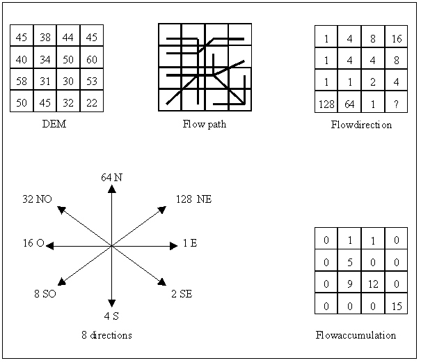
Figure 1: Grid functions for terrain analysis for hydrologic
purposes.
The stream and watershed network is determined so that there is a single
stream segment for each watershed that is modeled. The DEM cells that form
the streams are defined as the union of two sets of grid cells. The first
set consists of all cells whose flow accumulation is greater than a user-defined
threshold value. This set identifies the streams with the largest drainage
area, but not necessarily with the largest flow because flow depends on
other variables that are not related exclusively to topography. The second
set is defined interactively by the user by clicking a certain point on
the map, which results in an automatic selection of all downstream cells.
This tool was included in HEC-PrePro v. 2.0 because it was
observed that under specific circumstances users are interested on particular
streams, which might have a small drainage area (low flow accumulation).
To include these streams using the threshold criterion, it would be necessary
to lower the threshold value for the entire system, thus defining unnecessarily
a much more dense stream network.
Sub-basin outlets are also defined as the union of two sets of grid
cells. The first set, based on the stream network, consists of all cells
located just upstream of the junctions. Consequently, at a junction, two
outlet cells are identified, one for each of the upstream branches. The
system outlet is also identified as an outlet. The second set is defined
interactively by the user by clicking on any cell on the stream network
such as those associated with gages or other water control points. After
the sub-basin outlets have been defined, a unique identification code is
assigned to each stream segment connecting a headwater cell with a sub-basin
outlet, or two sub-basin outlets.
The watershed
GIS function is used to delineate the areas draining to each sub-basin
outlet. A one-to-one relation between stream segments and sub-basins is
maintained because a unique segment has been identified for each sub-basin
outlet.
Vectorization of the hydrologic elements
After the stream segments and their corresponding drainage areas have
been delineated in the raster domain, a vectorization process is performed
using raster-to-vector conversion functions included in ArcView Spatial
Analyst 1.1. This process consists of creating a line data set of streams,
and a polygon data set of sub-basins. The reason for this vectorization
is that the number of hydrologic elements (streams and sub-basins) in the
system is usually small compared with the number of grid cells, and further
processing and modeling is faster in the vector domain. Following the raster-to-vector
conversion, vector-processing steps are included to preserve the one-to-one
relationship between stream lines and sub-basin polygons, and to determine
the connectivity between polygons. When vectorizing sub-basins, it is important
to verify that each sub-basin is represented by a single polygon. A sub-basin
represented by more than one polygon is a common problem when the raster
representation of the sub-basin includes a dangling set of cells (a group
of cells that is connected to the main set of cells only through a corner),
because the raster-to-vector converter groups into discrete polygons cells
with the same value and a common side (see Figure 2). In such a case, the
dangling set of cells will be assigned to a different polygon, thus creating
a second polygon for the same sub-basin (same identification code). A program
has been included to merge all polygons � sometimes more than two �, that
correspond to the same sub-basin, into a single polygon.
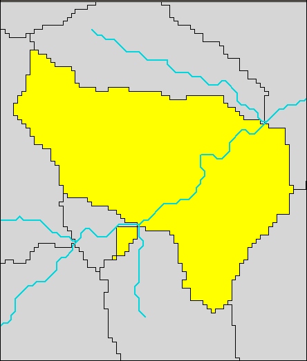
Figure 2: Watershed polygon with dangling polygons. Dangling
polygons are merged to the main watershed polygon by running an Avenue
script.
HEC-PrePro v. 2.0 also identifies, for each sub-basin
polygon, all the sub-basin polygons located upstream of it, and merges
them so that they can be easily retrieved when delineating a watershed
from a point, as will be explained below.
Computation of the hydrologic element parameters
The sub-basin parameters calculated by HEC-PrePro v. 2.0 are
area, length and slope of the longest flow-path, average curve number,
and lag-time. Since area and lag-time are the only parameters required
for the SCS dimensionless unit hydrograph, HEC-PrePro v. 2.0
is capable of generating all the necessary information for routing
flow in the sub-basin.
The sub-basin area is calculated automatically in the process of vectorizing
the sub-basin polygons.
The longest flow-path is identified as the set of cells of the sub-basin
for which the sum of the downstream flow length to the watershed outlet
and the upstream flow length to the sub-basin boundary is a maximum (Smith
1995). Before presenting other sub-basin parameters, it is important to
discuss the physical meaning of the downstream flow length to the watershed
outlet and upstream flow length to the sub-basin boundary. The downstream
flow length to the watershed outlet is equal to the distance along a flow
path from a grid cell to the outlet of the sub-basin in which it is located.
After running the (downstream) flowlength
GIS function -- which calculates the flow distance to the border of the
analysis window or to a nodata
cell (whichever is found first) -- the downstream flow length to the watershed
outlet is calculated as the difference between the flow length value of
the cell and the flow length value of its corresponding outlet cell. The
upstream flow length to the sub-basin boundary is equal to the distance
along a flow path from a grid cell to the most upstream location within
its watershed, and does not necessarily follow the main channel. After
assigning nodata
values to all sub-basin outlet cells, the (upstream) flowlength
GIS function -- which calculates the flow distance to the most upstream
cell of the analysis window or to a nodata
cell (whichever is found first) � is used to calculate the upstream flow
length to the sub-basin boundary. nodata
values are assigned to the sub-basin outlets to keep the flowlength
function from searching for longer flow-paths in the upstream sub-basins.
The length of the longest flow-path is equal to the maximum value of
the sum of the downstream flow length to the watershed outlet and the upstream
flow length to the watershed boundary.
The slope of the longest flow-path is determined as the elevation drop
between two arbitrarily defined points of the flow path, divided by their
distance along the channel. The points can be located at any user-defined
distance from the sub-basin outlet, expressed as a percentage of the length
of the longest flow-path. For instance, percentages of 10% and 85% refer
to that 75% portion of the channel located 10% of the channel length upstream
of the sub-basin outlet.
The average SCS curve number of the sub-basin is calculated as the average
of the curve number values within the sub-basin polygon. A curve number
grid is calculated using land use data described by Anderson's land use
code, percentage of each hydrologic soil group (A, B, C and D) according
to STATSGO soils data, and a look-up table that relates land use and soil
group with curve numbers (Smith 1995).
The sub-basin lag-time is calculated with the SCS formula and is given
by (Chow, Maidment and Mays 1988)
where tp (minutes) is the sub-basin lag-time -- measured
from the centroid of the hyetograph to the peak time of the hydrograph
--, Lw (feet) is the length of the longest flow-path, S (%)
is the slope of the longest flow-path, and CN is the average curve number
in the sub-basin. However, because in HMS the analysis time-step has to
satisfy the condition of being smaller than 0.29 times the lag-time of
the basin (HEC 1990), the lag-time is taken as the value given above or
3.5 times the analysis time-step, whichever is greater. Therefore, the
lag-time is redefined as
where Dt is the analysis time-step. Although
this modification artificially delays the flow in the sub-basin, it only
affects the very small watersheds (with lag-times smaller than 3.5 times
the analysis time step) in which the volume of runoff produced is small
compared with the size of the entire system. Moreover, mass conservation
is not affected by altering the sub-basin lag-time.
The stream parameters determined by HEC-PrePro v. 2.0 are
the length, the routing method � either Muskingum or pure lag --, the Muskingum
K and the number of sub-reaches into which the stream is subdivided in
case Muskingum is used for routing, and the flow time in case pure lag
is used for routing. Other stream parameters like the flow velocity and
the Muskingum X can not be computed by HEC-PrePro v. 2.0 and
must be calculated externally and supplied as input.
The reach length is determined automatically in the process of stream
vectorization, and flow time is calculated as  ,
where L is the reach length and v is the flow velocity.
,
where L is the reach length and v is the flow velocity.
The Muskingum method is used for stream routing in all reaches long
enough not to present numerical instability problems. In short reaches,
in which the flow time is shorter than the time-step, the pure lag method
is used as will be explained later.
To avoid numerical instability when using the Muskingum method, long
reaches are subdivided into shorter equal-length sub-reaches, so that the
flow-time in each of them satisfies the condition  (Fread 1993), where k is the flow time in the sub-reach. Since the flow
time in the sub-reaches is equal to
(Fread 1993), where k is the flow time in the sub-reach. Since the flow
time in the sub-reaches is equal to  ,
where K is the flow time in the reach, and n (an integer value greater
than zero) is the number of sub-reaches, then it follows
,
where K is the flow time in the reach, and n (an integer value greater
than zero) is the number of sub-reaches, then it follows
Moreover, because n should be at least equal to 1,
should be greater than Dt to satisfy the Muskingum
method constraints, otherwise the pure lag method must be used. Additionally,
the minimum number of sub-reaches into which the reach can be subdivided
is given by:
where int takes the integer part of the argument (int does not round
the number).
K for the Muskingum method and the lag time for the pure lag method
are both equal to the flow time which, as indicated above, is .
3.2. Isolation and process of a hydrologic sub-system
Isolation of a sub-system
Once the pre-process is done, the user may choose to isolate a hydrologic
sub-system for further modeling. A program has been included to isolate
the drainage area of a user-defined point, thus defining a sub-system composed
of streams and watersheds, and creating the corresponding GIS vector data
layers. Hydrologic element parameters -- computed as part of the pre-process
-- are tranferred to the attribute tables of the new data layers, and new
parameters are determined for the most downstream polygon.
Programs borrowed from the Watershed Delineator use the sub-basin polygon
data set created in the pre-process to speed up the watershed delineation
from a point. HEC-PrePro v. 2.0 identifies the sub-basin
polygon in which the user-defined point is located, isolates the DEM cells
for that polygon, performs the raster-based watershed delineation within
the polygon, and merges all the sub-basin polygons located upstream.
Topologic analysis and preparation of an HMS basin
file
After the vector data layers of the sub-system have been created, HEC-PrePro
v. 2.0 is used to transfer geographic information to the HMS basin
file. Considering all nodes in the stream network, the node classification
scheme developed by Hellweger and Maidment (1997) is used to identify junctions
and sinks. Junctions and sinks also serve as sub-basin outlets in HEC-PrePro
v. 2.0 because of the way in which stream lines and sub-basins are
defined. The connection between a sub-basin and its associated outlet is
determined by the proximity of the outlet point to the sub-basin polygon
boundary. The appropriate stream lines are identified as reach elements
depending on the node types at the beginning and end of each line.
As an intermediate step in the creation of the HMS basin file,
symbolic point and symbolic line coverages are created. Fields in the symbolic
point and symbolic line attribute tables store information about the connectivity
among elements and computed hydrologic attributes. Information from these
fields is written to the HMS basin file.
4. Application to the Llano
River in Central Texas
HEC-PrePro v. 2.0 has been run for the Llano River, tributary
of the Colorado River in Central Texas. A study area of 200 Km (North �
South) by 180 Km (West � East), which also includes the Concho and San
Saba Rivers, was identified (see Figure 3). A total of 145,000 500-meter
DEM cells were used in the terrain analysis.
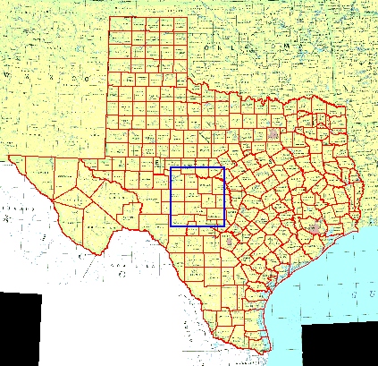
Figure 3: The study area is located in Central Texas and
includes the Concho, San Saba and Llano Rivers, tributaries of the Colorado
River.
The pre-process of the study area consists of running in sequence all
the options of the pull-down menu shown in Figure 4, from Fill Sinks to
Calculate Attributes. The process of a sub-system consists of running the
Run HECPREPRO option after isolating the sub-system.
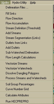
Figure 4: HEC-PrePro pull-down menu. Options should be run
in sequence.
After running the terrain analysis � Fill Sinks, Flow Direction, and
Flow Accumulation �, all cells draining more than 750 Km2 (3,000
grid cells) were identified as stream cells, and six additional streams
and one sub-basin outlet were added interactively. Figure 5 shows the streams
defined by the threshold criterion (blue), those added interactively (red),
and the sub-basin outlet (green).
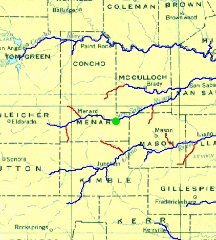
Figure 5: Streams and sub-basin outlets can be added interactively.
Blue streams have been defined by the threshold criterion, red streams
and the green sub-basin outlet have been added by clicking on the map.
Once streams and outlets are identified, sub-basins are delineated in
the raster domain. Figure 6 shows the resulting stream - watershed delineation
after vectorization, in which the Concho River, San Saba River, and Llano
River can be identified at the Northern, Central and Southern part of the
study area respectively.
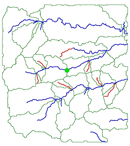
Figure 6: Stream - watershed delineation after vectorization.
Note the one-to-one relation between streams and watersheds.
Finally, hydrologic parameters for each of the elements are calculated
and attached to their corresponding attribute table, as can be seen in
Figures 7 and 8.
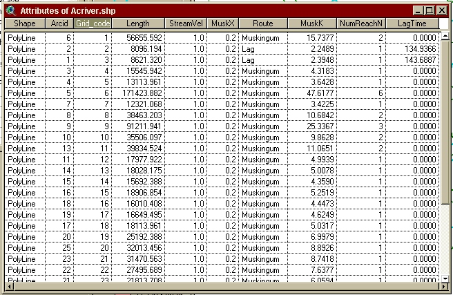
Figure 7: Attribute table of the stream vector data set.
Stream parameters have been attached to the table.
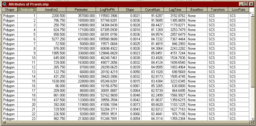
Figure 8: Attribute table of the watershed vector data set.
Watershed parameters have been attached to the table.
After isolating the Llano River basin by clicking near its junction
with the Colorado River, a basin file -- readable by HMS -- is created
using the information of the hydrologic system obtained in GIS. This basin
file, in ASCII format (Figure 9), includes the hydrologic parameters
of the elements, and their interconnectivity.
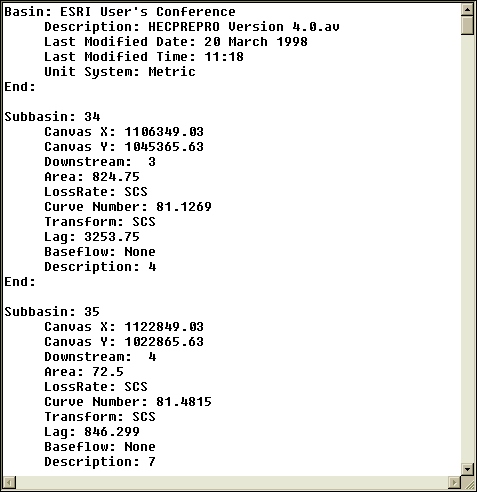
Figure 9: HMS basin file in ASCII format. Hydrologic
parameters calculated in GIS and stored in the attribute tables are transferred
to the basin file.
Figure 10 shows the schematic of the Llano River basin in the HMS -
Schematic window, and Figure 11 shows hydrologic parameters in the HMS
� Basin Model Editor window.
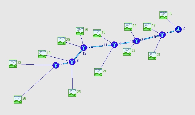
Figure 10: HMS display of the schematic of the Llano River
basin.
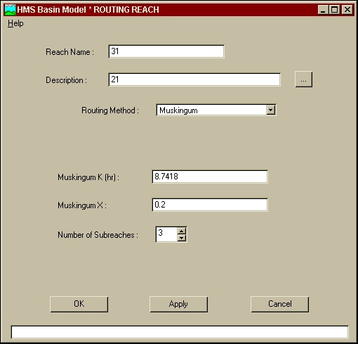
Figure 11: HMS element editor window. Stream parameters calculated
in GIS have been transferred to HMS.
5. Conclusions
A connection between GIS data sets describing a hydrologic system and
HEC's Hydrologic Modeling System (HMS) has been developed and called HEC-PrePro
v. 2.0.
HEC-PrePro v. 2.0 extracts hydrologic, topographic and
topologic information from digital spatial data, and prepares a basin
file in ASCII format, which when opened by HMS automatically creates
a topologically correct schematic network of sub-basins and reaches, and
attributes each element with selected hydrologic parameters. At the moment,
HEC-PrePro v. 2.0 is capable of determining parameters required
by the Soil Conservation Service (SCS) curve number method for loss rate
calculations, the SCS unit hydrograph model for watershed routing, and
either the Muskingum or pure lag method for flow routing in the streams
(depending on the reach length).
Using HEC-PrePro v. 2.0, the determination of physical parameters
for HMS is a simple and automatic process that accelerates the setting
up of a hydrologic model and leads to reproducible results.
In the future, HEC-PrePro v. 2.0 will consider other hydrologic
elements defined in HMS such as reservoirs, diversions and sources (system
inlets).
Acknowledgements
Development of HEC-PrePro v. 2.0 has been funded by the
Hydrologic Engineering Center (HEC) of the United States Army Corps of
Engineers and the Texas Department of Transportation (TxDOT). The contribution
of Zichuan Ye and Dean Djockic, developers of the Watershed Delineator,
Ferdinand Hellweger, developer of the code of HEC-PrePro v. 1.0, and Brian
Adams, who helped to put together the code of HEC-PrePro v. 2.0,
is greatly appreciated.
References
Chow, V.T, D.R. Maidment and L.W. Mays (1988), Applied Hydrology,
McGraw-Hill Inc., New York, 1988.
DeVries, J.J., and T.V.Hromadka (1993), Computer Models for
Surface Water in Handbook of Hydrology, ed. by D.R. Maidment, McGraw-Hill
Inc., New York, 21.1-21.39.
D.L.Fread (1993), Flow Routing in Handbook of Hydrology,
ed. by D.R. Maidment, McGraw-Hill Inc., New York, 10.1-10.36.
HEC (1990), "HEC-1 Flood Hydrograph Package," User's
Manual, p.24, Hydrologic Engineering Center, U.S. Army Corps of Engineers,
Davis, CA.
Hellweger, F., and D.R.Maidment (1997), Definition and Connection
of Hydrologic Elements Using Geographic Data, accepted for publication
in the ASCE � Journal of Hydrologic Engineering.
Jensen, S.K., and J.O. Domingue (1988), Extracting Topographic
Structure from Digital Elevation Data for Geographic Information System
Analysis, Photogrammetric Engineering and Remote Sensing 54 (11).
Jensen, S.K. (1991), Applications of Hydrologic Information
Automatically Extracted from Digital Elevation Models, Hydrologic Processes
5(1).
Smith, P. (1995), Hydrologic Data Development System, Master
Thesis, Department of Civil Engineering, University of Texas at Austin.
USGS a, 7.5-Minute Digital Elevation Model Data, http://edcwww.cr.usgs.gov/glis/hyper/guide/7_min_dem
as of March 1998.
USGS b, 1-Degree Digital Elevation Models, http://edcwww.cr.usgs.gov/glis/hyper/guide/1_dgr_dem
as of March 1998.
USGS c, Metadata for GCIP Reference Data Set (GREDS),
http://nsdi.usgs.gov/nsdi/wais/water/gcip.HTML
as of March 1998.
USGS d, Global 30 arc-second Elevation Data Set, http://edcwww.cr.usgs.gov/landdaac/gtopo30/gtopo30.html
as of March 1998.
Author Information
Francisco
Olivera, PhD
Research Associate
University of Texas at Austin
Center for Research in Water Resources
J.J.Pickle Research Campus # 119
Austin, TX 78712
Telephone: (512) 471-0570
FAX: (512) 471-0072
folivera@mail.utexas.edu
Seann
Reed
Graduate Research Assistant
University of Texas at Austin
Center for Research in Water Resources
J.J.Pickle Research Campus # 119
Austin, TX 78712
Telephone: (512) 471-0073
FAX: (512) 471-0072
seann@mail.utexas.edu
David Maidment,
PhD
Professor of Civil Engineering
University of Texas at Austin
Center for Research in Water Resources
J.J.Pickle Research Campus # 119
Austin, TX 78712
Telephone: (512) 471-0065
FAX: (512) 471-0072
maidment@mail.utexas.edu