Non-Linear Surface
Interpolations:
Which Way Is The Wind Blowing?
ABSTRACT
Geographic Information System
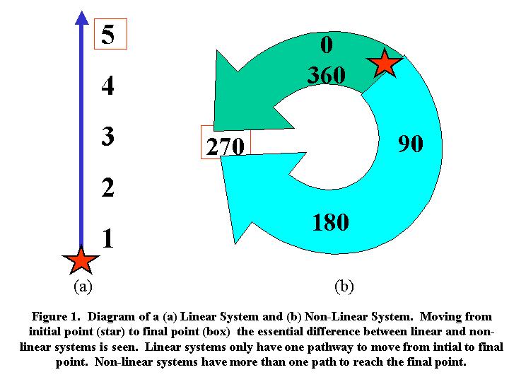
(GIS) surface interpolations are pure linear calculations, but many nonlinear
geographic phenomena exist in the real world. A compass, with 360 degrees,
describes a nonlinear situation. The same final direction may be reached by
moving in either a clockwise or a counterclockwise direction. How can nonlinear
conditions be modeled in linear-restricted programs? Translation functions may
be used successfully, but care must be taken when designing the model.
Potential conflicts and sign problems await the unwary GIS analyst. This paper
uses the specific example of calculating two-dimensional wind directions over
flat terrain to illustrate the pitfalls and pinnacles of nonlinear
interpolations.
1.0 INTRODUCTION
While interpolating wind fields between weather monitoring
stations, a series of difficulties were encountered due to the non-linear
nature of wind direction. This paper discusses the specific problems and
solutions found while programming the ArcView script and during subsequent
model testing. Non-linear scripting issues will share certain characteristics
and this discussion may assist others to avoid certain pitfalls while working
toward specific application solutions. Throughout this endeavor, three distinct
perspectives were needed to successfully create the non-linear model - that of
a technical expert, a mathematician, and obviously, a GIS analyst.
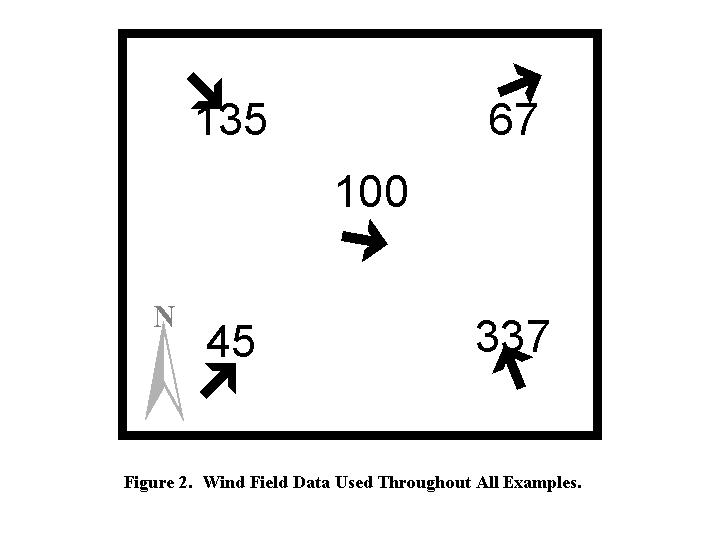
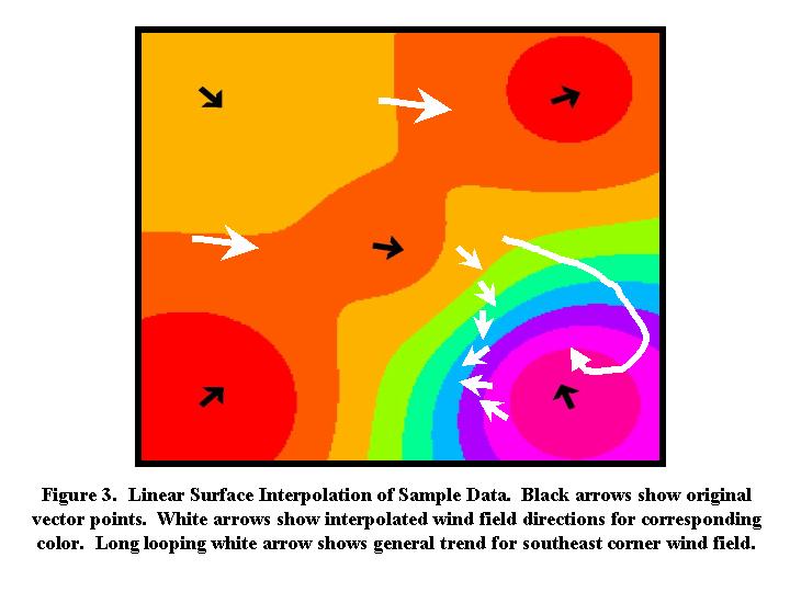
Using the sample data set, a linear ArcView Spatial Analyst
surface interpolation is run with results shown in Figure 3.
Generally, the results agree with our basic understanding of what should happen
for both the north and west sections. However, results in the southeast section
do not agree with our basic understanding. The black arrows are the original
monitoring station wind directions and the short, white arrows give the general
wind direction corresponding to each interpolated wind direction range color.
As can be seen in the southeast corner, the arrows rotate linearly. The long
looping arrow demonstrates how the wind supposedly curls about itself, rotating
through almost 270o, before matching the monitored wind direction.
Because of our basic understanding of what the interpolated wind field should
be, we know this result is not correct.
3.1 Non-Linear Transformations
The first thing to realize is a non-linear transformation
involves a good deal of math - so get over any math anxiety you may have. While
the transformation is complicated, the issues that arise are more from the
quantity of details rather than from complexity of the math itself. For our
specific example, high school level geometry and trigonometry are used. Other
applications could use higher levels of mathematics such as calculus or Fourier
transforms. The type of math used in the transformation depends upon the
specific application.
Terminology differences between the physical phenomenon
being modeled and the GIS environment can be an obstacle when modeling
non-linear characteristics. For the example winds, there is a difference
between the National Weather Service wind data and the vectors used within the
model. Not only are directions calculated differently, but they mean completely
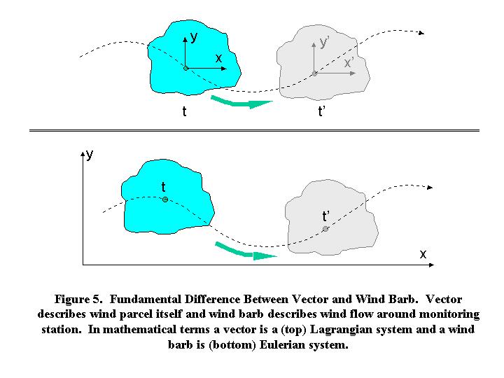
different things, Figure 4. A vector gives magnitude
and direction from a single arrow symbol. The length of the arrow corresponds
to the vector's magnitude, which in our example is wind speed. The arrow's
direction, measured counterclockwise from the right horizontal, gives wind
direction. A wind barb is actually three symbols combined and may be
interpreted to provide a variety of data, (Lutgens and
Tarbuck, 1995). The small circle describes the cloud cover condition, such
as clear or obscured skies. The long line tells whether there is any wind and
the direction from which it is blowing. The small lines on the end of the long
line give the approximate wind speed. Direction the wind is blowing is measured
clockwise from the vertical.
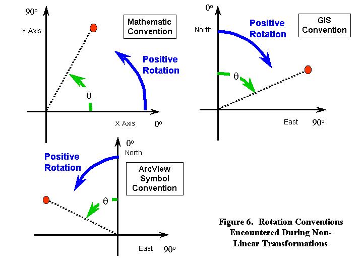
As mentioned in the introduction, different perspectives are
necessary for successfully modeling a non-linear phenomenon. One of the first
issues to be faced is rotation convention differences, Figure
6. For the three conventions shown, each has perpendicular axes that point
toward the east or x-axis, and the north or y-axis. From a pure mathematical
perspective, positive rotation is typically measured counterclockwise from the
x-axis. GIS convention positive rotation is clockwise from the y-axis. Care
must be taken when designing equations to consider these differences. Within ArcView
itself, rotation discrepancies exist. Symbol rotation in the ArcView menu Window/Show
Symbol Window is counterclockwise from the positive y-axis, exactly
opposite normal GIS rotation convention.
|
Radians |
Degrees |
|
0 |
0 |
|
p/4 |
45 |
|
p/2 |
90 |
|
p |
180 |
|
2p |
360 |
Convention differences play an important role when designing a GIS model. As can be seen, depending on the perspective at any time during model troubleshooting, conflicting conventions can cause confusion.
4.1 Pure Mathematics
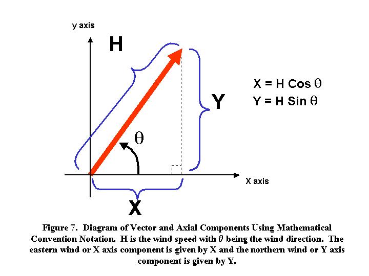
The best transformation is a simple transformation. Analyze your specific non-linear situation for simple mathematic substitutions. Simple is best because it typically limits the number of details you will encounter. For our specific example, one vector at each monitoring site gives two pieces of information-wind speed and wind direction. Wind speed is linear and does not need transformation. Wind direction is non-linear and must be transformed.Using geometry, a vector can be separated into axial components, Figure 7. The magnitude of the vector is represented by the variable H and the direction is given by q. The axial components are given by
|
X = H Cos q |
(1) |
|
Y = H Sin q |
(2) |
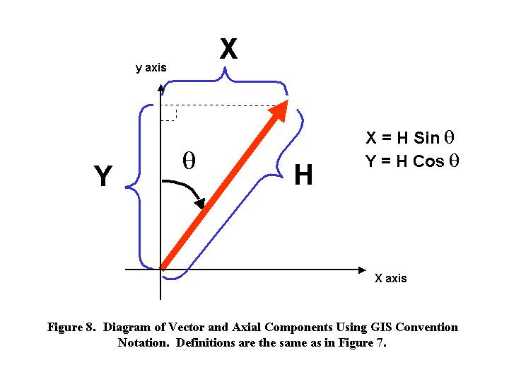
Because of convention differences between pure mathematics and GIS, equations (1) and (2) must be compared and transformed into GIS conventions. While pure mathematics define the transformation formulas, the angle and rotation definitions must conform to GIS standards. Because of the operating environment ArcView, the angles used by the ArcView math functions use GIS conventions. To illustrate this point, Figure 8 diagrams the mathematical transformation situation shown in Figure 7 in GIS normal conventions. Of importance is not only the difference in rotation but the change in the formula. The equations actually reverse! The GIS convention corrected transformation equations are
|
X = H Sin q |
(3) |
|
Y = H Cos q |
(4) |
This is a good example why documenting process analysis and transformation equations are important. In addition, an excellent visualization tool is graphing diagrams of all relationships. This is especially advantageous in the areas of rotation conventions. If equations (1) and (2), were used for the ArcView linear analysis, the results would be unrealistic. Therefore, when creating a non-linear surface interpolation, be sure to transform the mathematically derived equations into GIS conventions.
At this point, the non-linear wind vector has been
successfully transformed into linear vector components in the x and y
directions. Normal ArcView Spatial Analyst surface interpolations may be used
to create interpolated wind fields - one for the northern wind component and
one for the eastern wind component. Within ArcView, multiple types of linear
interpolations are possible. This paper does not present comparisons between
the interpolation types; references that provide general information on this
subject include Hu and Isaaks. Different interpolation types lend themselves to
various applications.A later section in this paper does provide a comparison
and details potential decisions that a scriptwriter will make.
6.0 TRANSFORM LINEAR COMPONENTS BACK INTO NON-LINEAR FORM
6.1 Pure Mathematics
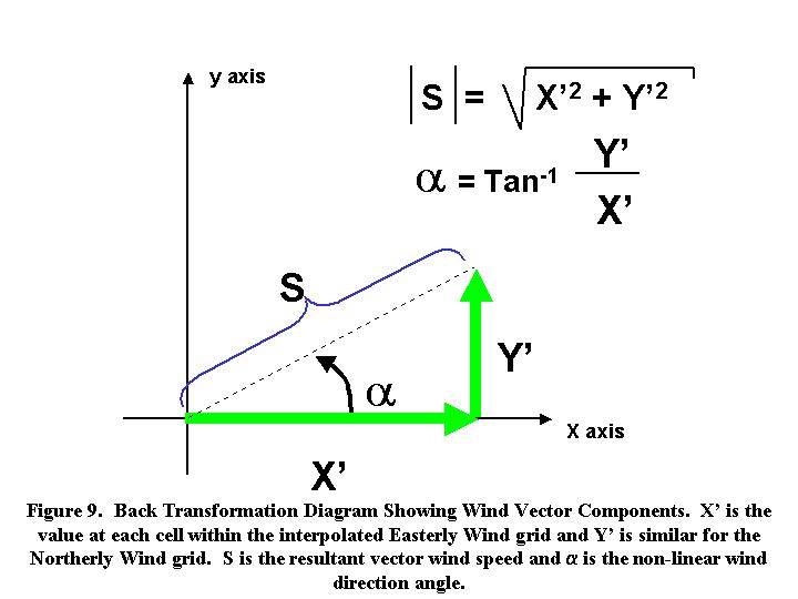
The desired result of the script is a non-linear interpolated wind field.At this point, we have two separate grids, northern wind and eastern wind. Each grid gives an axial wind component value for the same grid cell location.In Figure 9 the northern wind is designated Y’ and the eastern wind is X’. To combine the wind components into the desired result involves mathematical calculations. From geometry, the magnitude of the vector, the wind speed, is calculated as
|
|S| = (X’2 + Y’2)1/2 |
(5) |
and the vector direction or wind direction is given by
|
a = Tan-1(Y’/X’) |
(6) |
Note equation (5) has an absolute value. Does this
complicate the back transformation? No, it does not. No matter if X' and Y' are
positive or negative, the resultant wind magnitude is always positive due to
the squaring of the component vector terms. So how does ArcView know which way
the non-linear wind vector should point?The wind direction, equation (6),
provides that information. Once again, determining the angle involves careful
consideration due to its non-linear nature. We will work through each non-linear
issue for the back transformation. From the initial transformation efforts, we
know to check the mathematically derived equations against GIS conventions.
However, before doing this step, additional concepts must be introduced.
It is important to know the signs of the wind component
vectors because they indicate the positive or negative axis direction. Figure 10 illustrates a single vector with axial
components. Depending on the vector’s quadrant, the axial components take on
different signs. Quadrants are geometric nomenclature that define sections
within the graph and are designated by roman numerals in the figure. Quadrant I
is bounded by the positive x and y axes and both vector components are positive.
Quadrant II is bounded by the positive x and the negative y axes with the
eastern wind component being positive and the northern wind component being
negative. Similarly, Quadrant III is bounded by the negative x and y axes and
both wind components are negative. The fourth quadrant is bounded by the
negative x and the positive y axes and the vector components follow the same
sign convention. The significance of the quadrant and sign conventions will be
evident shortly.
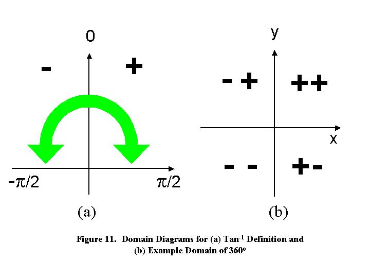
Complications arise from equation (6) due to computer math
function limitations and not due to convention conflicts. Figure
11(a) shows the domain that defines the inverse tangent, Tan-1,
trigonometry function. Results are only valid between -p/2 and p/2; this
is only half of the domain we need, Figure 11 (b).
Therefore, including wind component signs is irrelevant because with or without
them, the mathematic model does not encompass the full domain of the GIS
region. The inelegant solution involves two steps - calculate wind direction
based on absolute values, then rotate the angle to the correct quadrant.
However, this solution does not work for all quadrants. Calculated values are
only valid for the first and third quadrants. If a Quadrant I angle is simply
rotated by 270o to translate into Quadrant IV, it is obvious why the
simple translation does not work, Figure 12. Angles in
the fourth quadrant are "mirror images" of the first quadrant angles
and it can be proved that the fourth and second quadrant formulas are the same
with a simple rotation needed for quadrant corrections. The same method as in
Section 4.2 will be used to diagram angles and check derived equations. The
solution to the problem is interesting and involves angle symmetry.
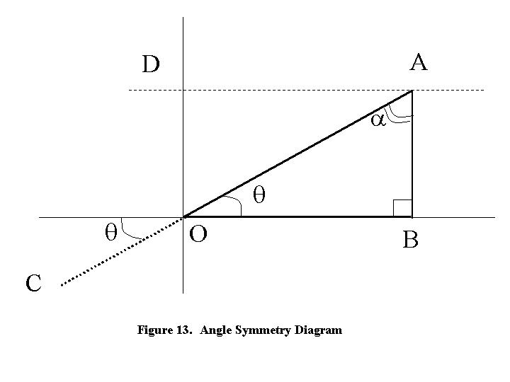
Within geometry, certain rules govern certain geometric shapes. Within a triangle, the sum of all interior angles always equals 180o. If one angle is a right angle, equal to 90o, then the sum of the remaining angles is also 90o. Therefore, from Figure 13, we know
|
q + a = 90o |
(7) |
The angle q is defined by the lines AOB and a is defined by the lines OAB. If lines OB and DA are parallel, then the triangle OAB and ODA have the same included angles. Therefore, the angle defined by DAO is equal to q and the angle AOD equals a. This is also demonstrated by the fact that line AB is perpendicular to both lines OB and DA. A right angle is defined by the lines DAB. If a is included within angle DAB, then from (7)
|
q = 90o - a |
(8) |
So it is possible to identify angles based on symmetry using known angles and parallel lines. Angle DAO equals q and angle AOD equals a. This can be extended to other quadrants. For example, Quadrant III of Figure 13 gives q by symmetry using the horizontal axis and line COA. Therefore, the angle defined by the line CO and the vertical axis must equal a. It is left to the reader to investigate angle symmetry within the other quadrants. Angle symmetry can be used to re-diagram quadrants two and four; only Quadrant IV is shown, Figure 14.Quadrant II is re-defined similarly.Derived equations for each quadrant to back translate wind direction are given below. Once again, we see a reversal in equations to reach our desired answer. Within the ArcView script, a conditional “If statement” that uses wind component signs will allow the model to select the correct equation.
|
Quad I |
q = Tan-1(X’/Y’) |
(9) |
|
Quad II |
q = Tan-1(Y’/X’) + 90o |
(10) |
|
Quad III |
q = Tan-1(X’/Y’) + 180o |
(11) |
|
Quad IV |
q = Tan-1(Y’/X’) + 270o |
(12) |
As discussed earlier, be sure the trigonometric function is working with radians, rather than degrees at this point. The trigonometric functions in ArcView will not recognize degrees. You may use a conversion such as p/180 to convert from degrees to radians within the script or the database information may be modified before beginning actual calculations.
7.0 THE LAST CHECK
7.1 Sanity Checks
Finally, the last check relies on a scriptwriter's ability
to understand the phenomenon that is being modeled. Each time a transformation
glitch is fixed, it is important to give the results a "sanity
check". Always use test data. By knowing the answer before the computer
finishes crunching the numbers ensures rapid analysis of the results and
facilitates positive progress with model development. Test data specific for
each quadrant should be used before checking a general test model. As discussed
earlier, the different quadrants present analysis and programming challenges
that must be addressed within a successful model. By using test data specific
to each quadrant, it is possible to check the equation results to ensure the
diagramed angles discussed earlier are correctly interpreted. By using the
different perspectives of technical expert, mathematician and GIS analyst,
sanity checks are quick methods to see if the programming is proceeding in a
positive direction. A technical expert understands the trends of the phenomenon
being modeled. A mathematician tests formulas with data where the correct
answer is already known.And a GIS analyst is key to developing the
methodology.Together, these different disciplines give the multidiscipline
knowledge needed to create a non-linear interpolation script.
7.2 Interpolation Types and the Effects on Non-Linear
Models
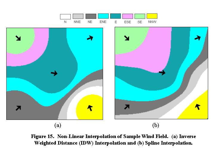
Once the non-linear model successfully interpolates the
data, two non-linear grids will define a single vector. One grid gives wind
speed, magnitude, and the other gives wind direction. Figure
15 shows the non-linear interpolation of wind direction for the sample data
set. As discussed in the previous section, technical expertise is important to
develop the best non-linear model possible. For those not familiar with
atmospheric science, Figure 15 (a), may look
acceptable. However, wind does not typically move so that "blobs"
occur in the wind field. Note the corners and center of the figure which show
large areas of the same general direction with relatively quick changes of wind
direction between the "blobs". Figure 15 (b)
gives a better interpretation of a wind field. These two diagrams use the same
sample dataset, Figure 2, but give different results
due to the interpolation technique used during the linear portion of this
process. As discussed in Section 5.0, the type of linear interpolation used
affects the outcome of the non-linear interpolation model. Figure
15 (a) was calculated using the Inverse Distance Weighted (IDW) method
which "assumes that each input point has a local influence that diminishes
with distance", (Esri, 1996). This method
restricts the values at all points to always being within the bounds set by the
monitoring site points. Figure 15 (b) used the Spline
technique that fits a "minimum curvature surface" through the data
points. This method allows "gently varying surfaces" to be modeled
and does not restrict the maxima and minima within the interpolated field.
8.0 CONCLUSIONS
It is possible to perform non-linear surface interpolations within a linear restricted GIS program such as ArcView with Spatial Analyst extension. Geometry and trigonometry are involved and the potential exists for higher level mathematics depending on the specific application. The most difficult obstacles are convention conflicts and detail confusions that can be overcome with proper documentation and diagramming. By using test data where the desired outcome is known, model comparisons can be performed rapidly. Sanity checks and using quadrant specific test data facilitates non-linear model development. Finally, during script development, troubleshooting issues from the three perspectives of technical expert, mathematician and GIS analyst will give insights to the pitfalls involved with non-linear surface interpolations within a linear restricted GIS program.
Thanks go to Dr. Jim St. John of Georgia Tech for pointing out the obvious during the initial stages of model development. It's amazing how dependent we become on technology to solve all our problems when sometimes going back to the basics gives the best results.
ArcView v3.1 and Spatial Analyst v1.1 were used for this project.
An air parcel is the atmospheric equivalent of a water drop or dirt clump.
Batchelor, G.K., 1994. An Introduction to Fluid Dynamics. Cambridge University Press, New York, 615 pp.
Esri, 1996. ArcView Spatial Analyst, Environmental Systems Research Institute, Inc., Redlands, 147 pp.
Hu, J., 1995. “Methods of Generating Surfaces In Environmental GIS Applications”, 1995 International Users Conference. Environmental Systems Research, Inc.
Isaaks, E.H. and Srivastava, R.M., 1989. Applied Geostatistics. Oxford University Press, New York, 561 pp.
Jacobson, M.Z., 1999. Fundamentals of Atmospheric Modeling. Cambridge University Press, New York, 656 pp.
Kvaal, A., Sanders, J. and Walikis, R., 1998. “Kodak Air Resources Evaluation System 2000 (KARES 2000): Air Quality Management using ArcView Geographic Information System”, Esri International User Conference. Environmental Systems Research Institute, San Diego California.
Lutgens, F.K. and Tarbuck, E.J., 1995. The Atmosphere: An Introduction to Meteorology. Simon & Schuster Company, Englewood Cliffs, New Jersey, 462 pp.
Patterson, W., 1997. “Integrating ArcView and the Spatial Analyst Extension with the PRISM Climate Expert System”, Esri 1997 International Users Conference. Environmental Systems Research Institute, Inc., San Diego, CA.
Rabayda, A.C., 1997. “Air Force Combat Climatology Center (AFCCC) Applications of ArcView GIS and ArcView Spatial Analyst”, Esri 1997 International Users Conference. Environmental Systems Research Institute, Inc, San Diego, CA.
Shipley, S.T. and Graffman, I.A., 1998. “ArcView GIS is a Weather Processing System”, Esri International User Conference. Environmental Systems Resource Institute, San Diego, California.
Shipley, S.T., Graffman, I.A., Beddoe, D.P. and Smith, M., 1997. “Rapid Integration of COTS GIS for Interactive Weather Processing”, 13th International Conference on Interactive Information and Processing Systems (IIPS) for Meteorology, Oceanography, and Hydrology. American Meteorological Society, Atlanta, GA.
Tchepel, O., Borrego, C. and Barros, N., 1997. “Using GIS in MesoScale Atmospheric Modeling”, Esri 1997 European GIS Users Conference. Environmental Systems Research Institute, Inc.
van
der Wel, F.J.M., 1997. “Introducing GIS Technology at the Royal Netherlands
Meteorological Institute”, Esri International User Conference. Environmental
Systems Research Institute, San Diego California.
AUTHOR INFORMATION
|
Environmental Engineer 1777 Hardee Avenue ATTN:AFPE-ENE Fort McPherson, GA30330-6000 fax:(404)464-7827 e:mail:williaro@forscom.army.mil |
Georgia Institute of Technology School of Earth and Atmospheric Science Atlanta, GA 30332 |