Mapping and Analysis of Pennsylvania's Telecommunications Infrastructure
Guoray Cai, Kenneth M. Sochats, and James G. Williams
Department of Information Science and Telecommunications
School of Information Sciences
University of Pittsburgh
135 N. Bellefield Avenue
Pittsburgh, PA 15260
(ABSTRACT)
State and local governments have a need to understand the spatial distribution of telecommunications infrastructure and services in order to plan for a competitive information economy and for universal services. This paper presents Pennsylvania's (link-to-learn) experiences in the comprehensive mapping of state-wide telecommunications infrastructure using Esri's GIS technology. Problems of data integration, representation and models for the assessment of telecommunications infrastructure are discussed, together with proposed solutions based on spatial modeling techniques. Based on the techniques acquired and generated, an interactive mapping server has been developed (using MapObjects) to facilitate sharing and usage of this public information.
1. Introduction
Recent advances in high capacity optical fiber, digital transmission and switching, wireless, and satellite technologies are believed to be the major driving forces for the ongoing information revolution [2] in cyberspace. The digitization of human interaction and social mediation through telecommunications has created an environment that is having profound influences socially, culturally, economically, and geographically in this new world of cyberspace. [5, 16, 33]. It is believed that the technological infrastructure of a geographical area will determine how well it survives in the 21st century in much the same manner that the road, water, and electrical infrastructure determined how well states survived in the 20th century. This infrastructure includes telecommunications, transportation, utility, land, and institutional facilities (medical, safety, etc.) as well as the human knowledge and skills infrastructure.
In 1996, Pennsylvania initiated a $132 million dollar project called "Link to Learn" with the goal of using information technology to improve the quality and quantity of education in the Commonwealth K-12 schools. The use of advanced telecommunications facilities and services to access cyberspace to achieve this goal for improving education underlies the link to Learn initiative. In order to determine where to invest funds and encourage infrastructure development to support the goal and build access to cyberspace, it was determined that the technology infrastructure of the Commonwealth needed to be documented. This documentation was to result in an on-line, Web accessible database and a Web accessible Geographic Information System (GIS). The purpose of each was to permit an analysis of where the gaps in technology infrastructure existed in the Commonwealth for the purposes of investment, development, and policy formulation. The database contains technology data (hardware, software, LANs, WANs, Telecommunications, etc.) from over 11,000 organization sites including 6,237 educational sites, 1555 libraries, 186 telecommunication companies, 757 governmental sites, 159 utility company sites, 1,215 general businesses, 212 Internet Service Providers, 567 medical facilities, and others. As the name of the initiative implies, the anchor tenant of infrastructure support for education is telecommunication facilities and services. Therefore, an emphasis was placed on documenting this infrastructure as completely as possible at the physical and logical network level. Wire center and inter-wire center backbone network data was collected from the incumbent local exchange carriers (ILECs), the inter-exchange carriers (IXCs), competitive local exchange carriers (CLECs), competitive access providers (CAPs), and cable companies operating in Pennsylvania. A data set was also purchased that contained all the wire centers in Pennsylvania. Although the data is not complete, approximately 80-90 percent of the infrastructure data has been amassed. All the telecommunication infrastructure elements have been coded using the state plane coordinate system. Wire centers are treated as point data elements, circuits are treated as lines segments and service areas are treated as polygons.
In contrast to the position that considers the use of telecommunication technologies and cyberspace to be 'placeless' or 'anti-spatial', others suggest that space and location continue to play important roles in understanding the cyberspace phenomena. Kitchin [14] presented three major reasons in support of this position.
Among all the components of information technology, telecommunications infrastructure exhibits the strongest ties to geography. The infrastructure elements are carefully located to reach geographically distributed customers as much as possible. They tend to persist in their location for long periods of time, and all the service provision and consumption activities are organized around these infrastructure facilities.
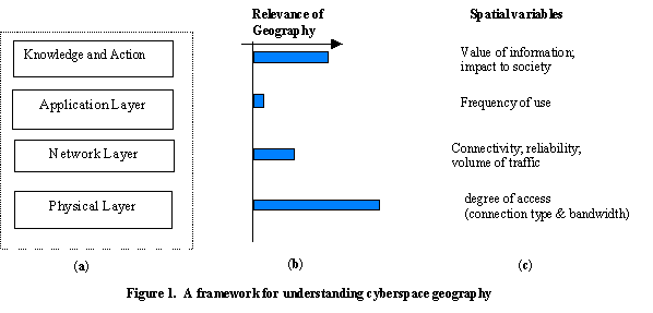
The telecommunication infrastructure and its associated cyberspace can be considered to be multi-layered, with each layer showing different type of spatiality (See Figure 1). Four layers can be identified that have distinct geographical properties: physical layer, network layer, application layer, and knowledge and action layer. In understanding the relative importance of geography in the study of each layer, the bar graph on Figure 1b is helpful. In such a framework, the above arguments are no longer contradictory since they deal with the spatial properties of cyberspace in different layers.
At the physical layer, the distribution of telecommunications infrastructure and the concentration of service providers is highly biased by geography. This results in spatial variations in the types of available services and access bandwidth. At the network layer, a set of locations can be minimally connected or maximally connected, depending on the reliability requirements and traffic characteristics. The application layer is the least sensitive to geographical locations, since it doesn't matter where one logs in to run a network application. Although, geographical location becomes relevant when the network application is run to support a business process that is located in a specific place. This is where the 'spaceless' position holds most of its truth. The 'knowledge and action' layer refers to the fact that information exchanged in the virtual space needs to be integrated into the user's knowledge or to induce some real-world actions which generate different local effects.
Most of the existing studies about the geography of cyberspace have been focused on the top layer. For example, the geography of information economy is concerned with the restructuring of the economic landscape in response to development of telecommunications technologies [30, 6, 15]. Social geographies of cyberspace have asked many geographical questions relating to community, democracy, privacy, access and exclusion [13, 21]. On the other hand, there has been lack of empirical and theoretical work that have derived formal properties of cyberspace in the physical and network layers.
This paper will present some GIS approaches to the study of the telecommunication infrastructure or cyberspace geography at the physical and network layers. At the physical layer, the bandwidth of access is mapped as a surface from telecommunications infrastructure information using a spatial model that combines ‘proximity’ and ‘distance decay’ transformations. In modeling customers' proximity to the nearest infrastructure elements, Voronoi diagram algorithms are used to define the ultimate region of influence of each infrastructure element. The distance decay effects of metallic twisted pair access technologies is modeled by a buffering transformation that is a commonly available GIS tool. The results from this type of spatial modeling can be directly applied to practical problems such as discovering gaps of infrastructure in a region (also called ‘gap analysis’) and detecting significant bias in the distribution of infrastructure elements. At the network layer, we used a family of planar graph models (nearest neighbor graph, minimum spanning tree, relative neighbor graph, Gabriel graph, and Delaunay triangulation) for the study of fiber connectivity pattern among a set of locations.
Although collecting the data was a difficult problem, a more imposing problem was the fact that the data came from multiple sources in different media, units of measurement, scales, geographic coverage, temporal coverage, spatial data types, error characteristics, projection type, and degrees of abstraction. In addition, some of the data to be associated with the telecommunication infrastructure elements came from a completely different conceptual domain. For instance, characteristics of elements such as schools, libraries, and hospitals differ radically from the characteristics of telecommunication infrastructure elements but needed to be integrated to show where gaps existed and to allow decision making based on a spatial representation. For instance, overlaying a map of technologically poor school districts with telecommunication networks and services can show where the telecommunication infrastructure and services need to be expanded or enhanced. An additional problem arises in selecting how to represent the infrastructure elements and the best method of producing a visualization that can convey conceptual information in a spatial domain.
We implemented our WEB accessible database using an NT platform, MS Access, MS SQL Server, Active Server Pages and Visual Basic 6.0. The WEB accessible mapping service was implemented using Arcview, Map Objects, and Visual Basic.
2. Telecommunications
2.1 Infrastructure
Telecommunications networks, which provides access, transport, switching, and signaling functions for the process of information exchange, is the core component of modern technology infrastructure. We make distinctions between infrastructure facilities and non-infrastructure facilities in telecommunications networks. The term "telecommunications infrastructure", or "TI", is used here to refer to those elements of telecommunications systems that are highly shared, carrying high volume telecommunications traffic, and, in most cases, spanning large geographical distance. Examples of telephone infrastructure include LEC’s inter-office networks, IXC’s backbone networks, and their switching equipment. In contrast, non-infrastructure network elements refer to facilities that are not shared and that are usually local extensions or value-added customizations of the infrastructure elements. According to this definition, all the local loop circuits, whether they are plain telephone lines, advanced DSL lines, or even fiber loops, are all non-infrastructure elements because they are not publicly shared.
Because of their shared nature, telecommunications infrastructure components can achieve enough economy-of-scale so that they can be equipped with the most advanced technology, and have almost unlimited capacity. Technology innovations, such as scalable design and Wavelength Division Multiplexing (WDM), have made it easy for a digital, fiber based infrastructure to meet the growing demand for high capacity without significant expansion or reconfiguration. For example, many circuits can be multiplexed onto the same fiber depending on the terminal and repeater technologies used. Therefore, by changing the terminal and repeater technology, a carrier can significantly increase its capacity without installing new fiber due to increased optical channels at different wavelengths. In some cases, carriers have deployed newer fiber called "dispersion shift fiber" to support multiple wave length technologies.
As telecommunications networks become totally digital, it is now possible that a single digital telecommunications infrastructure can serve many diverse sets of information services that were traditionally served by separate data, voice, and video networks. Modern telecommunications networks show a clear trend towards an all-fiber, all-digital infrastructure. In the meantime, networks of different types and owners are increasingly interconnected and integrated to expand their geographic reach. Based on such observations, there has been the vision of interoperable information infrastructures at the global, national, local and enterprise levels [23]. Unlike traditional infrastructures which are public utilities offering a limited and monopolistic service and operating in a stable market structure, the new telecommunications industry is able to provide a host of different services and products, and operate in a highly competitive market system [29].
We will limit our discussion to two types of infrastructure elements, wire centers and fiber routes, although there are many other types of infrastructure related to microwave, wireless, and satellite communications technology. Wire centers are places where digital switches are hosted, and they are major access points for subscriber loops and interconnection points among facilities of different providers. Optical fiber has penetrated both the backbone access and local area network where it replaces classical coaxial cable or twisted pair networks. Due to its unlimited bandwidth, its immunity against electromagnetic interference, its very low losses (below 0.5 dB/km) it has become the preferred transmission medium for long distance or high bit-rate connections.
2.2. Twisted Pair Based Loop Technologies
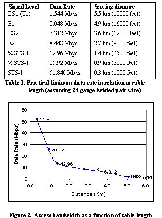
It is becoming increasingly clear that telephone companies are going to utilize existing twisted-pair loops in their next generation broadband access networks [28]. This is largely due to the technology advance in high bandwidth modem systems which are able to convert twisted pair telephone lines into access paths for multimedia and high-speed data communications. Horak [11] provided a discussion of a group of advanced twisted pair local loop technologies in terms of bandwidth and distance limitations. Among these access technologies, Asymmetric Digital Subscriber Line (ADSL) and its variants such as Very high rate Digital Subscriber Line (VDSL), etc. are believed to be the most viable broadband solution to most customers. An ADSL circuit connects an ADSL modem on each end of a twisted-pair cable, creating three information channels: a high- speed downstream channel, a medium speed duplex channel, and a voice channel. It depends upon advanced digital signal processing and creative algorithms to squeeze as much information as possible through twisted pair wires. It is a repeater-less technology, which means that no significant reengineering work is needed to install ADSL service on an existing twisted pair loop. VDSL employs essentially the same set of techniques as ADSL, but is designed to deliver much higher bandwidth over shorter distance. The variations of ADSL/VDSL can be considered as a continuum, a set of transmission tools that delivers about as much data as theoretically possible over varying distance of twisted-pair telephone wires. Table 1 provides a summary of various data rates available on a 24 gauge twisted pair wire. The relationship between access bandwidth and distance to the serving wire center is shown in Figure 2.
3. Data Integration and Representation Issues
3.1 Data Integration
Data integration refers to the process of combining layers of map data by visualizing composite displays of different types or by using integration models that create a new map from two or more existing maps. This requires matching similar entities in the sources and having information consistency across the data sources. GIS map overlay operations are used to relate different types of geographical features based on spatial relationships such as point by point, point in polygon, intersects, crossing, neighbor of, and outside of. In addition to inconsistencies in spatial data their may also be inconsistencies in attribute data as well. Table 2 shows a classification of the different consistency issues.
|
Operation |
Spatial Consistency |
Conceptual Consistency |
|
Display Consistency |
Coordinate system, coverage, and scale |
Not required |
|
Overlay (point-to-point composite) |
Data Model, entity type, scale, coordinate system, coverage |
Not required |
|
Overlay (Point-to-point comparison) |
Data model, entity type, scale, coordinate system, coverage |
Required |
Table 2. Consistency Classification Issues
Spatial data integration requires two steps to remove the inconsistencies. The first step is to resolve the inconsistencies and the second step is to use one or more of the GIS spatial overlay operations to interrelate the consistent data to meet the application requirements. The methods used to create consistent spatial data sets are shown in table 3.
|
Spatial Data Technique |
Attribute Data Technique |
|
Map Projection Conversion Geometric Rectification Feature Generalization Scale Conversion Raster to Vector Conversion Conversion to Zonal System Spatial Aggregation Surface Interpolation Co-registration of Maps |
Aggregation of Data Subclasses Reclassification Reduction in Numeric Precision Reduction of level of measurement Conversion to Common Database Schema Attribute Normalization |
Table 3. Consistency Resolution Techniques
Multiple data integration issues for two spatial data sets can sometimes be resolved by taking a one-at-a-time approach but this will not always work. It is sometimes better to deal with 2 or more inconsistencies at the same time.
An example of the data integration issue with telecommunications might be where one data set has fiber routes and digital switch locations represented as lines and points respectively and a second data set describes customer locations and their service demand as an attribute by application type such as e-commerce, distance education, video conferencing, etc. The conceptual attributes of these two data sets are not comparable. But, by converting the fiber and digital switch locations in the first data set to "access bandwidth" and the applications in the second data set to demand bandwidth, we have a comparable attribute for each data set which we can combine into a third data set for purposes of producing a composite map. The transformation for both maps must ensure that all spatial entities in the composite data set have a matching entity in the first and second data sets. A graphical representation of this consistency resolution process is shown below.
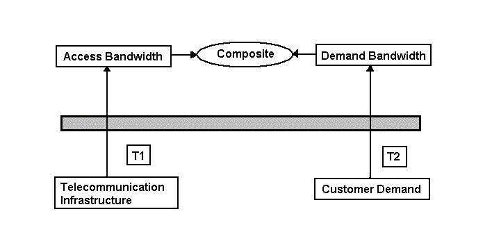
Figure 3. Data Integration Transformation
3.2 Representation
Spatial coordinate data collected for the telecommunication infrastructure elements covered a wide range from the state plane system and latitude and longitude to street addresses and the telephone industry's H and V coordinate system. These were all converted to the state plane system for consistency. Likewise, data may be represented as points, lines, or areas (polygons). And each of these may transformed from one type to another. Table 3 shows the elementary transformations that may need to be used to make two spatial data sets consistent.
|
From/to |
Points |
Lines |
Areas |
|
Points |
Interpolation (1) |
Contouring (2) |
Thiessen ploygons(3) |
|
Lines |
Line Intersections(4) |
Line Smoothing(5) |
Buffer Zoning(6) |
|
Areas |
Sample points(7) |
Medial Axis(8) |
Re-Sampling at area(9) |
Table 3. Representation Transformations
(1) Spatial interpolation from one set of points to another set of points
(2) Joining points of equal value with iso-lines
(3) Generating Thirssen or Voronoi polygons from irregularly distributed points
(4) Find intersection points where lines cross
(5) Making a smoother line from a digitized line by "weeding" vertices
(6) Dilation of lines to create corridors at a specific radii
(7) Append area attributes at points to a point attribute table
(8) Each polygon is reduced to an outline or medial axis line
(9) Convert the attribute values of one set of polygons to another set of polygons such as population by county to population by congressional district
Selecting the appropriate basic representation for the telecommunication infrastructure elements is not as difficult as determining what representation is best for analysis or a visualization to convey a concept. Once a representation is selected, then the required transformation must be applied if the basic representation if different from the basic one. A simple example is where a wire center 's base representation is a point but must be converted to an area such as a circle to represent an access related concept. The more difficult situation is where there is more than a single element with different representations and they must not only be integrated but the appropriate representation must be selected as well. For example, if the percent of a county with access to fiber optic cabling is to be visualized, then the fiber circuits represented as lines might be converted to areas using a buffer zone transformation and the county represented as a polygon or area might be colored according to the ratio of land area of the county and the land area covered by the buffered fiber circuit. In this case, the size of the buffer zone is determined based on technological concepts. There are many such types of analyses and visualizations that require more than a single transformation.
4. Mapping the Geography of Telecommunications for Link To Learn
Although a large number of analyses and visualizations were performed for the Link To Learn project using spatial analysis methods only 2 will be covered here in detail, namely broadband access and gap analysis. Pennsylvania is a largely rural state with the largest rural population of any state in the US. Pennsylvania also has a large number of incumbent facility based telephone companies (36), all the major long distance carriers, and over 40 alternative telecommunication providers not counting the 400 cable franchises. In addition, many utility companies have installed fiber optic cables along their rights-of-way. The inequality of access to advanced telecommunications services is well recognized in the literature [26]. Such inequality can be attributed to the geographically biased distribution of telecommunications infrastructure and the biased distribution of service providers. But, the future telecommunications market will be based on a facility-based competition model, hence the factor of service providers will fade out. For such reasons, telecommunications infrastructure will be the primary determinant of the geography of access. In the same time, the capability of the infrastructure in a region will be better understood if it is translated into the magnitude of communication bandwidth that the infrastructure could provide to each location in the region.
4.1. Assumptions
In order to establish a quantitative relationship between the distribution of telecommunications infrastructure and the geographical variation of access, we make the following assumptions:
(1). Facility-based market competition.
Market competition among different service providers will be totally based on the quality and spatial reach of their facility. Recent regulatory changes, as indicated by the Telecommunications Act of 1996 [24] have moved telecommunications market towards true competition, and service barriers like price distortion, lack of profit, and service boundaries are likely to be removed partially or totally.
(2). The capacity of infrastructure elements can be considered as unlimited.
With the scalable design and multiplexing technologies, the capacity of the existing digital switches and fiber circuits can be increased to meet the growing demands without significant reconfiguration.
(3). Majority of the access circuits will remain twisted pair metallic cables within the near future.
These assumptions allow us to model the geography of access based solely on spatial information about wire centers and fiber optic cables in a region. The assumption (1) means that the access bandwidth of a location is dependent only on its distance to the nearest infrastructure elements. The assumption (2) makes the case that we do not need to know the capacity of individual infrastructure elements as long as we know that they are digital switches and fiber cables. The assumption (3) implies that the access bandwidth of a location is constrained by the electrical characteristics of twisted pair metallic wires. In general, longer wires will induce more signal impairment, and hence less effective bandwidth available in the communication channels.
4.2. A Model of Access to Telecommunication Infrastructure
Based on the assumptions, a model was developed that will derive the access bandwidth of every location in a region that is served by a set of wire centers and a set of fiber optic cables. The model is based on nearest neighbor and distance decay principles and is fully implemented in the Arcview GIS system. In order to given a formal description of the model, the following notations is used:
R: a region representing the study area.
WC: a set of points within R, representing the location of wire centers serving that region.
FO: a set of line segments within R, representing the location of optical fiber cables.
C: a set of points within R, representing a group of customers (for example, schools, libraries, and hospitals)
Wc(r): the wire center nearest to r
Fo (r): the fiber cable nearest to r
Î RNND(r, WC): the distance from r
Î R to Wc(r), the nearest wire center.NND(r, FO): the distance from a point r
Î R to Fo (r), the nearest fiber cable..Bwc(d): the characteristic function of copper wires that represents the deliverable bandwidth as distance decay function of the distance to nearest wire center.
BFO(d): the characteristic function of copper wires that represents the deliverable bandwidth as distance decay function of the distance to the nearest fiber optic cable.
Then, the access bandwidth, A(r), of any point r in a region R can be represented by:
A(r) = Maximum { Bwc( NND(r, WC) ), BFO( NND(r, FO) ) }
In order to calculate A(r) for a point r in a GIS, these are the steps:
(1). Calculate the Voronoi diagram for all the wire centers and for all the fiber routes. This can be done using the point and line Voronoi diagram algorithms described in [19, 3, 20]. Clipping the Voronoi diagrams with the boundary of region R;
(2). Derive Wc (r) and Fo(r) by a ‘point-in-polygon’ test. A wire center Wc is the nearest to the location r only if r is within the Voronoi region of Wc. Same way to find the nearest fiber cable;
(3). Calculating the nearest neighbor distances NND(r, WC) and NND(r, FO);
(4). Calculate A(r) using formula (1).
Since a value of A(r) can be calculated for every location in the region R, the model will result in a three dimensional surface which predicts the access bandwidth of any location from the spatial distributions of wire centers and fiber cables.
4.3 Application of the Model
The model we suggested can be used for two kinds of studies.
Throughout the discussion of applications, we will use the data set shown on Figure 4 for illustrative purpose. The data set is the partial result of the large-scale survey conducted by the State of Pennsylvania [25, 32] in its Link To Learn
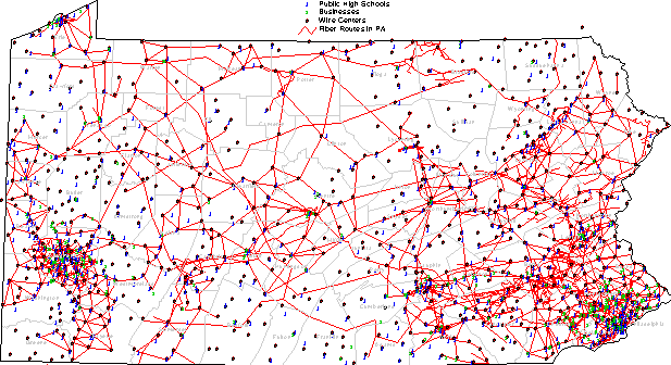
initiative. It shows the locations for two types of telecommunication infrastructure elements(the wire centers and fiber optic cables) and two types of customers (major businesses, and public high schools) within the State. Figure 5 shows the result of applying the model of access to the wire centers and fiber optic cables. In figure 5a, the green, white, and orange colors represent areas that have broadband, wideband, and narrowband access, respectively. Similar interpretation can be made to figure 5b.
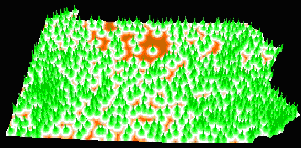
(a). Access Bandwidth deliverable from Wire Centers

(b). Access Bandwidth deliverable from Fiber Optic Cables
Figure 5. Surface Model of Access Bandwidth
4.3.1. Redefining Spatial Relations
Spatial relations of telecommunications do not correspond to geographical relations in a simple way. For example, you no longer ‘go to’ a ‘place’, but you 'call' or ‘log in’ onto the net. So the traditional concepts of ‘distance’ and ‘nearby’ no longer directly apply. But we argue that the variations in access bandwidth generate a feeling of ‘distance’, because the higher the bandwidth, the shorter the time to wait for large transactions to complete. In this sense, the concept of ‘near’ between two entities can be redefined according to the maximum capacity of the communication channel they can set up for exchanging information. Using the example in figure 5, the virtual distance between locations a and b can be expressed as: (assuming that all the wire centers are connected by optical fiber networks)
VD(a, b) = minimum ( A(a), A(b) )
This provides the possibility to quantitatively define and map those virtual entities, such as ‘virtual community’, or ‘virtual school’.
4.3.2. Gap analysis.
Telecommunications consumption activities may be associated with spatial point objects in the geographical space, such as households, schools, libraries, supermarkets, and office buildings. When the existing infrastructure can not support the desired services from the consumer points, we say that the infrastructure has ‘gaps’, or ‘holes’, with it. But the discovering of these gaps can not be simply done by counting the number of facilities (e.g. number of wire centers or length of fibers) in a particular area. The model proposed in figure 6 could provide a formal approach to this task.
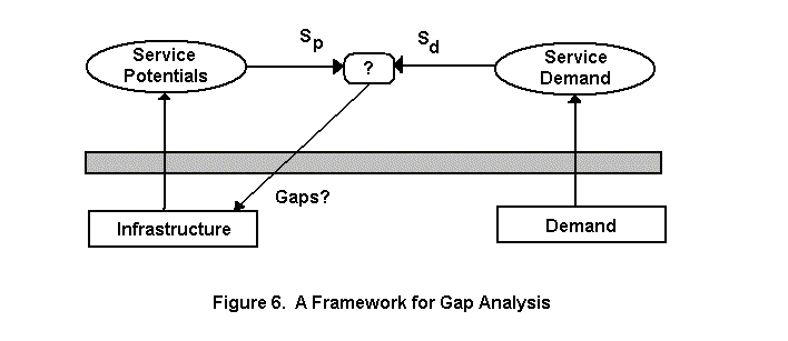
For convenience, these points will be referred to as consumption points, or C-points. We may characterize each C-point by three measures: Existing service (Se) refers to the current usage of any telecommunications services; Service potential (Sp) refers to the maximum possible telecommunications capacity that current infrastructure is capable of delivering to the C-point; service demand (Sd) is the total need of telecommunications capacity. All three variables are dynamically changing and interacting with each other over time. Whenever (and wherever) Sp is lagging behind Sd, it is an indication of less than adequate infrastructure. Figure 5 shows the relationships of these variables.
For example, suppose that all the public high schools in the State of Pennsylvania are expected to exchange courses through high quality distance learning networks, which requires at least T1 (1.544 Mbps) connection. By spatially sampling the value of surface in Figure 4 with the location of those schools, the gaps in infrastructure can be identified by comparing the required bandwidth with the bandwidth predicted by the model.
4.3.3. Detection of Bias.
The telecommunication infrastructure tends to be geographically biased towards major metropolitan areas and business centers, compared to the relatively sparse facilities in rural and less developed areas where the demand is marginal [31]. Such biased pattern occurs because that the acquisition of these facilities requires huge capital investment, that it is only economically feasible in areas of high existing (and/or projected) demand. Castells [6] suggested that telecommunications technologies are actually reinforcing urban hierarchies through the processes of restructuring. In the process of spatial reorganization, corporations actively locate and relocate their control centers in areas with suitable infrastructure in order to take advantage of the global reach of telecommunications technologies. The telecommunication industries, in turn, are attracted by major business centers where they can reach large number of customers within a small geographical area.
Telecommunications infrastructure is not only biased by geography, but is also biased towards serving certain categories of consumers. For example, Figure 4 shows a pattern that the existing infrastructure in the state of Pennsylvania is strongly biased towards businesses comparing to schools. There are many reasons for such a pattern to occur. First, businesses have been historically the earliest and strongest demands for telecommunications services, and the telecommunication industries have been attracted to businesses as a source of customers. In contrast, other customers, such as schools, libraries, churches, area located to serve residential areas, and may historically have relatively small influence on the location of infrastructure elements. This means that an existing infrastructure that support the networking of businesses may be found inadequate to support an educational network which connect all schools, libraries, and homes. If such bias is found to be significant in a region, then public policies and government investment must be designed to correct infrastructure bias
As an example, both types of bias are clearly shown in the map of Figure 4. This has significant implications in the geography of access to telecommunications services. It is in this sense that the spatial distribution of telecommunications infrastructure determines the landscape of access. Biased existence of telecommunications infrastructure contributes to the geographic unevenness in terms of access to advanced telecommunications services. While the biased pattern does exist, the degree of such bias varies from region to region in the state, and we need a method to test the hypothesis for a given area. Since the degree of such bias may vary from region to region, and from one type of consumer to another, there is a need to statistically test the significance of such bias.
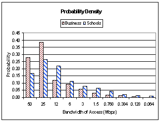
Figure 7. Probability Distributions in relation to access bandwidth
Here we suggest a method to test the significance of bias based on the surface model of access. Figure 7 shows the result of sampling the access surface in Figure 5a by two separate point sets: public high schools and businesses. Let f(u) and g(u) represent the probability density function of businesses and schools, respectively. We can detect significant bias by testing the Null hypothesis that the net effect function:
e(u) = f(u) - g(u) = 0
The result of
c 2 test on the data in Figure 7 shows significant bias of wire centers towards serving businesses.5.0 Mapping the Geographical Variations at the Network Level
Telecommunications networks can be modeled as planar graphs in order to study their connectivity patterns. To measure the network connectivity of the telecommunications infrastructure, one can take two approaches. First, one could measure various properties of the underlying network graph, such as the number of intersections per unit area, number of circuits formed by edges in the graph, or frequency distributions. Second, one could compare the telecommunications network with models of graph line patterns. The second approach is shown here.
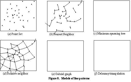
In Figure 8, a variety of models of line patterns are shown in order of increasing connectivity. A minimum spanning tree (MST) is defined as a tree having a set of edges such that the sum of lengths of all the edges is a minimum over all trees with the same point set. Scott [22] gives an iterative approach for building MST by connecting the disconnected segments of the nearest neighbor graph, which is a subgraph of the MST. As telecommunication networks rarely use a tree topology because of a lack of redundancy in a tree, Figure 8(d)(e)(f) show three examples of circuit models.
Gabriel graphs. For a given point set P, the Gabriel graph, denoted by GG(P), is defined by the graph in which ![]() is an edge of GG(P) if and only if the circle having
is an edge of GG(P) if and only if the circle having ![]() as a diameter is an empty circle [8]. Two points pi and pj are said to be Gabriel neighbors of each other if there is a direct link between them in the Gabriel graph.
as a diameter is an empty circle [8]. Two points pi and pj are said to be Gabriel neighbors of each other if there is a direct link between them in the Gabriel graph.
Relative neighborhood graph. This is a subgraph of the Gabriel graph. A relative neighborhood graph, denoted by RNG(P), is defined as a geometric graph in which RNG(P) has an edge between pi and pj if and only if
![]() [27]. In other words,
[27]. In other words, ![]() is an edge of RNG(P) if and only if there is no other point of P in the interior of the intersection of the two disks, one with center at pi and the other centered at pj, with the same radius
is an edge of RNG(P) if and only if there is no other point of P in the interior of the intersection of the two disks, one with center at pi and the other centered at pj, with the same radius ![]() . The relative neighborhood graph has the ability to extract perceptually relevant structures from sets of points
. The relative neighborhood graph has the ability to extract perceptually relevant structures from sets of points
Delaunay triangulation. This is a geometric dual graph of a Voronoi diagram, and can be constructed by joining those pairs of points pi and pj whose Voronoi regions have an edge in common. A Delaunay triangulation of a point set forms a space-exhaustive, contiguous tessellation of the planar space, and is locally and globally equiangular [19]. All circumcircles of delaunay triangles are empty circles. It is interesting to note that the Delaunay graph DG(P) of a point set P contains many other graph models as its subgraphs. Figure 9 shows a Delaunay graph and its four subgraphs for easy comparison. These graphs form a family of models for line patterns.
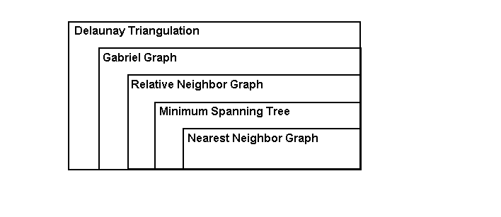
Figure 9. The Relationship Between the Delaunay Graph and Its Subgraphs
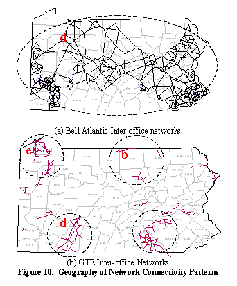
In any pattern of demand, there may be locations of demand that are spatially arranged in such a way that they are better connected by some network topologies than by others. There is an indication that natural connectivities have been used in practical network design. For example, Bell Atlantic has indicated that the Gabriel graph model of their wire centers in Pennsylvania (Figure 10a) is remarkably similar to the current topology of their inter-office network. Topology, which is either less dense, such as relative neighbor graphs, or denser, such as the Delaunay triangulation, would not be appropriate models of the network topology.
Figure 10b shows the best fit of models in figure 8 to each cluster of inter-office networks of GTE. Once such a model is developed, interesting questions of spatial hierarchies, subgraphs of clustered locations, or areas of under-or over-connectivity can be determined.
6.0 Summary
This paper demonstrates that GIS technology combined with a quantitative approach to the measurement of spatial properties of telecommunications networks can be used to analyze various aspects of the infrastructure. The spatial analysis approaches shown suggest several ways to measure the effectiveness and connectivity of a telecommunications infrastructure.
A geographical study of telecommunications infrastructure can significantly improve our understanding of the use of telecommunications networks and the resulting implications for the developing cyber communities. It can argued that cyberspace which is seen as an anchor tenant for the Link To learn initiative has a multi-layered organization and that at the lower, physical level telecommunications networks are not uniformly distributed in space. In turn, these inequities at the physical level result in fundamental, spatial differences in terms of the impact of telecommunications services required for cyberspace membership by society at large. Furthermore, the analytical tools of geographical information science provide the appropriate methodology for modeling the telecommunications infrastructure.
REFERENCES
[1] Adams, P. C., and Warf B., 1997, Introduction: cyberspace and geographical space. The Geographical Review, 87(2): 139-145.
[2] Adams, P. C., 1997, Cyberspace and virtual space. The Geographical Review, 87(2):155-171.
[3] Aurenhammer, F., 1991, Voronoi diagram - a survey of a fundamental geometric data structure. ACM Computing Surveys. 23, 345-405.
[4] Benedikt, M. (ed.), 1991, Cyberspace: first steps. Cambridge, MA:MIT Press.
[5] Burrough, P. A., 1986, Principles of Geographical Information Systems for Land Resources Assessment. Oxford University Press
[6] Castells, M., 1996, The Network Society. Oxford: Blackwell.
[7] Daniels, P., 1995, Services in a shrinking world. Geography 80, 87-110.
[8] Gabriel, K. R., and Sokal, R. R., 1969, A new statistical approach to geographic variation analysis. Systematic Zoology, 18, 259-278
[9] Graham, S., 1998, The end of geography or the explosion of place? Conceptualizing space, place and information technology. Progress In Human Geography. 22(2), 165-185
[10] Harvey, D., 1989, The condition of Postmodernism: an enquiry into the origin of cultural change. Oxford: Blackwell.
[11] Horak, R., 1997, Communications Systems and Networks. MIS:Press, Inc., New York.
[12] Hudson, H. E., 1997, Global Connections – International Telecommunications Infrastructure and Policy. Van Nostrand Reinhold, New York. ( 576p.)
[13] Jones, S. G., 1995, Introduction: from where to who knows. In: Jones, S. G. (ed.) Cybersociety: computer mediated communication and community. London: Sage, 1-9
[14] Kitchin, R, 1998, Towards geographies of cyberspace. Progress In Human Geography. 22(3), pp. 385-406
[15] Kitchin, R., 1997, Social transformations through spatial transformation: from ‘geospace’ to ‘cyberspaces’. In: Behar J. (ed.), Sociological studies of transformations, computerization and cyberspace, New York: Dowling College Press, 149-174.
[16] Laurini, R., and Thompson, D., 1992, Fundamentals of Spatial Information Systems. Academic Press, London
[17] Mitchell, W., 1995, City of bits: space, place and the infobahn. Cambridge, MA: MIT Press.
[18] Newton, P., Zwart, P., Cavill, M., Crawford, J. R., Edney, P., and Greener, S., 1991, GIS for telecommunications planning and management. In: Worrall, L., (ed.), Spatial analysis and spatial policy using geographic information systems. Belhaven Press, London. c1991. pp. 75-101.
[19] Okabe, A., Boots, B., and Sugihara K., 1992, Spatial Tessellation - Concepts and Applications of Voronoi Diagrams. John Wiley & Sons, Chichester, USA. 521p.
[20] Preparata and Shamos, 1985, Computational Geometry: An Introduction. Springer-Verlag, New York, USA. 390p.
[21] Schuler, D. 1995, Public space in cyberspace. Internet World. 6, 88-95
[22] Scott, A. J., 1971, Combinational programming, spatial analysis, and planning. London: Methuen.
[23] Targowski, A. S. , 1997, Global Information Infrastructure : the Birth, Vision, and Architecture. Idea Group Publishing, Harrisburg, USA.
[24] TA96, 1996, Telecommunications Act of 1996, Pub L. No. 104-104, 110 Stat. 56, codified at 47 U.S.C., 151 et. seq.
[25] Technology Atlas, 1998, Technology Atlas for a New Pennsylvania. available from
http://www.state.pa.us/pA_Exec/OIT/techinitiatives/atlas.htm[26] Thomas, R., 1995, Access and inequality. In: Heap, N. Thomas, R., Einon, G., Mason, R, and Mackay, H. (eds.), Information Technology and Society: a reader. Milton Keynes: Open University Press.
[27] Toussaint, G. T., 1980, The relative neighborhood graph of a finite planar set. Pattern Recognition, 12, 261-268.
[28]
Twisted Pair Access to the Information Highway. Available from URL: http://www.adsl.com/adsl_tutorial.html.[29] Vogelsang, I., and Mitchell, B. M., 1997, Telecommunications Competition: The Last Ten Miles. The MIT Press, Cambridge, MA. (364 p.)
[30] Warf, B., 1995, Telecommunications and the changing geographies of knowledge transmission in the late 20th century. Urban Studies, 32, 361-178.
[31] Williams, F., 1997, Telecommunications and economic development: a U.S. perspective. In: Chapter 3, Alexander, D. L. (ed.), Telecommunications Policy: Have Regulators Dialed the Wrong Number? Praeger Publishers, Westport, CT, USA.
[32] Williams, James G. & Kenneth Sochats, 1998, Electronic Commerce: Is Pennsylvania Ready. Technical Report, Department of Information Science and Telecommunications, University of Pittsburgh.
[33] Worboys, M., 1995, GIS, a Computing Perspective. Taylor & Francis, London.