David H. Graetz
Department of Forest Resources
College of Forestry
Oregon State University
ABSTRACT: Forest simulation models have been limited to non-spatial analysis or spatial analysis at aggregated scales. They have also traditionally neglected episodic disturbance processes such as wind, insects, and fire events. The Applegate River Watershed Forest Simulation Project is an attempt to achieve resource management goals by developing a model which reveals the outcomes of various management strategies while incorporating the interactions between the forest, fire, insects, wind, and social desires. In addition, the landscape parameters used in the model are maintained at a very fine resolution (25 meters) during the entire process. Heuristic programming techniques are used to reduce the computational time without compromising the detailed spatial analysis.
This paper gives an overview of the Applegate River Watershed Forest Simulation Project (hereafter called the Applegate Project). The goal of the Applegate Project is to develop a landscape simulation model for the Applegate Partnership (a collaborative planning group in the Applegate watershed), land management agencies, and others, to use in evaluating the potential effects of different policies and forest management practices to achieve goals for the watershed.
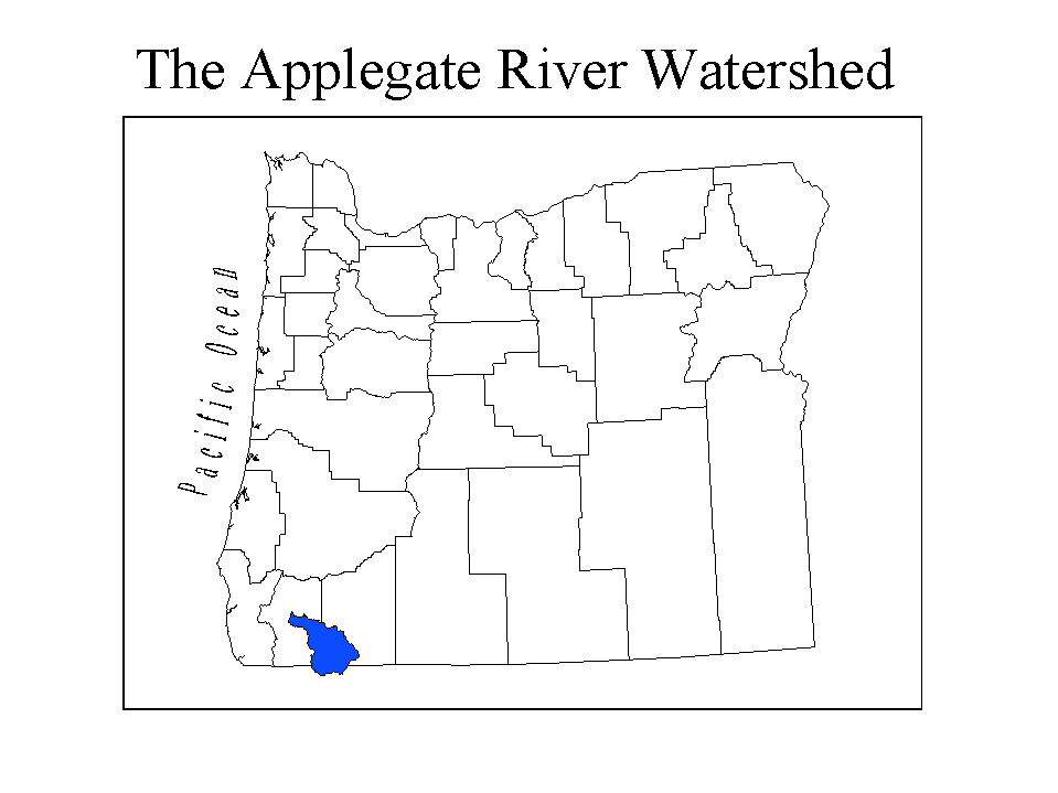
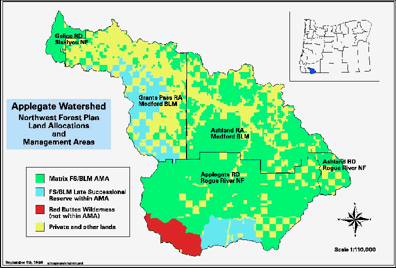
The Applegate River watershed is located in Southwestern Oregon (Figure 1). The watershed is approximately 493,000 acres and drains into the Rogue River. U.S. Forest Service and Bureau of Land Management (BLM) lands comprise nearly two-thirds of the ownership and contain almost 80% of the forested lands. The watershed's 325,000 acres of federal lands were designated an Adaptive Management Area (AMA) in 1994 with the signing of the Northwest Forest Plan (Figure 2). The remaining one-third of the watershed is in private ownership (mostly non-industrial). These lands generally occupy the valleys and lower elevations.
An ecosystem health assessment (USDI BLM et al., 1994) of the Applegate AMA found the following:
1. There is an increased risk of insect attack because of high stand densities.
2. A younger and denser stand make-up as compared to pre-European settlement.
3. Stocking levels exceed the carrying capacity over much of watershed.
4. There is an increased risk of fire because of increased fuel-loading and stand conditions.
Additionally, the AMA assessment contained some management recommendations and goals at both the stand and landscape level:
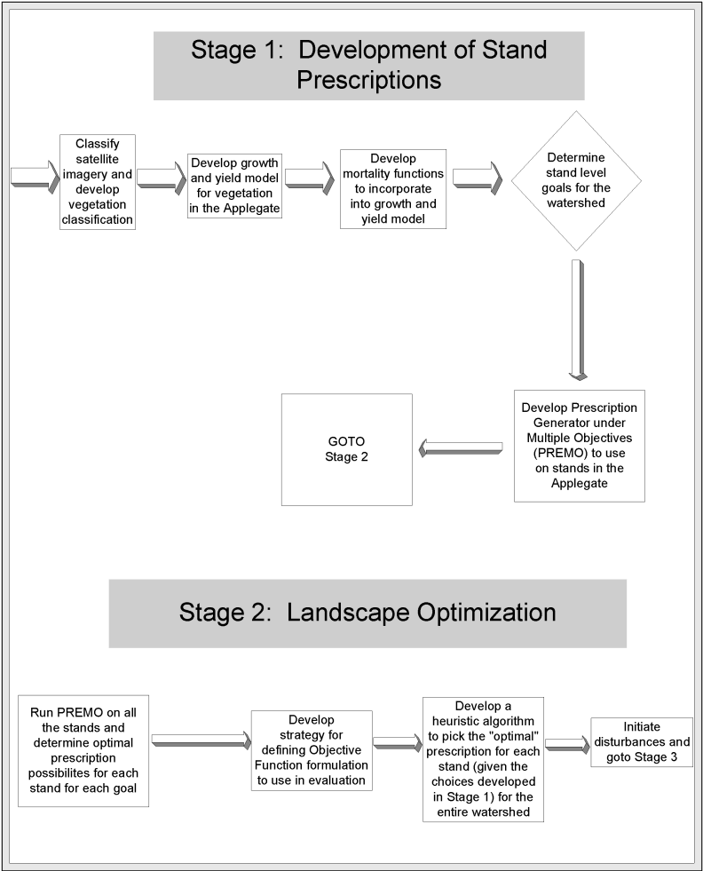
The Applegate Project has been designed to develop a simulation model to use in helping to achieve these goals. There will be three main components to the overall simulation model - a stand prescription optimization model, disturbance models (which include fire, insect, and wind-throw models), and a landscape optimization model. A four stage process will be developed to test the impact of different management approaches on the landscape over a long-term planning horizon (100 years):
(see Figure 3 and Figure 4 for an outline of the four stages)
Vegetation classes and seral stages for the watershed have been developed using Landsat TM satellite imagery captured in August, 1993. Thirteen vegetation classes (stand type) and fifteen seral stages (stand condition) are recognized within the watershed. The first stage of the modeling process will be the development of stand prescriptions, for each of the recognized stands in the watershed, that integrates growth, mortality, and achievement of goals. Growth relationships found in the Forest Vegetation Simulator (FVS) (Dixon and Johnson, 1995) serve as the foundation for a new stand prescription generator called PREMO (PREscription generator under Multiple Objectives) (Wedin, 1999). Periodic insect, wind, and root disease mortality will be incorporated into PREMO using relationships on decay of snags and down wood from Mellen and Ager's (1998) coarse woody debris model.
PREMO will be designed to take stand data, represented by a list of live trees, dead trees, and down woody debris (called a "treelist"), and create an array of prescriptions for the stand to reflect management goals. Five potential goals that have been developed by the Applegate Partnership are: 1) limiting fire hazard; 2) limiting insect and wind-throw hazard; 3) enhancing wildlife habitat; 4) improving fish habitat; and 5) providing a positive Present Net Value (PNV). The tools for manipulating stand condition in order to achieve goals are growth, tree harvest, and snag creation. Measurements of goal attainment are based on stand structural characteristics as calculated by investigating the modeled residual treelist (standing live and dead trees, and down wood) or the modeled harvest treelist. The RLS-PATH (Yoshimoto et al., 1990) optimization algorithm will be used to find prescription alternatives for each stand for each goal.
The planning horizon for the simulation project is 100 years, modeled as twenty, 5-year planning periods. Stage two is a two-phase process which includes the selection of specific prescriptions for every stand, and the start of the temporal movement of the landscape. The prescriptions developed by PREMO in stage one are optimized at the stand level based on stand goals. The idea in phase one of stage two is to optimize the selection of specific stand prescriptions based on landscape goals. Potential landscape goals include the same five stand goals mentioned earlier (limiting fire hazard, limiting insect and wind-throw hazard, enhancing wildlife habitat, improving fish habitat, and providing a positive PNV). Other potential landscape goals are those which are spatial in nature. Examples include ensuring X number of snags are left on every 40 acres; maintaining even-flow of timber in area Y while improving fish habitat in adjacent area Z.
A heuristic optimization algorithm will be developed to select the stand prescriptions initially assigned for the entire planning horizon. Heuristic programming is a broad term that describes a method of solving large, multi-variable, combinatorial optimization problems. Monte Carlo integer programming, simulated annealing, genetic algorithms, and tabu search are examples of heuristic algorithms (often just called heuristics). Heuristics find near-optimal solutions through various processes that allow the algorithm to employ a search or sampling strategy of the possible solutions. Some unique elements of heuristics include: 1) they do not look at all the possible solutions, 2) they may have some sort of "memory" which prevent the algorithm from continuously looking in one "area" for a solution, 3) they tend to have a set of rules that allows the algorithm to accept inferior solutions with the ideal that it may lead to a better solution, and 4) they are not guaranteed to find the mathematically optimal solution, in fact they may not find a solution at all.
The solution given by the heuristic will be a near-optimal solution to the underlying landscape question: "Which prescription do we choose for each stand (assuming the stand prescriptions alternatives have already been optimized) that optimizes the landscape given a set of landscape goals."
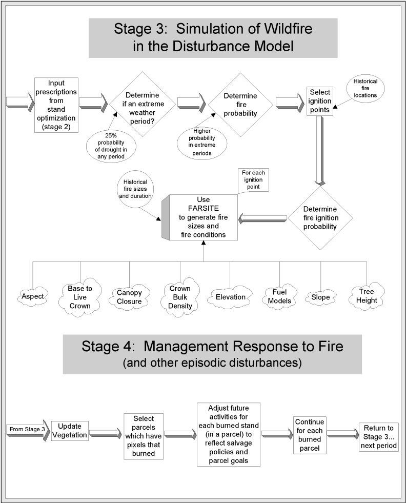
Once stand prescriptions are picked for period 0, those prescriptions will be assigned to stands for the entire 100 year planning horizon in the absence of episodic disturbance. The second phase of stage two relates to the temporal changes on the landscape. This means that the overall landscape model moves into the next period once all the landscape modeling processes for a period are finished. Stages three and four outline the two other landscape modeling processes that occur each period (again, the selection of stand prescriptions based on landscape goals is the first stage).
Periodic disturbance effects are incorporated in PREMO (stage one) but episodic disturbance will occur in stage three. Episodic disturbances will include fire, insect attacks, and wind-throw damage. Each of these disturbances will have a separate stochastic model that is spatially explicit. A fire-spread model called Farsite (Finney, 1998) will be used to initiate and spread a fire on the landscape. Probabilistic events such as the occurrence of drought will be taken into account when determining when and where fire occurs. Farsite will output flame lengths for any fire on the landscape and we will be able to associate the flame lengths with specific effects to a stand treelist.
The insect and wind-throw models are driven by relationships which describe which stands will be affected at what time. The occurrence of an insect or wind-throw event is a function of the weather, particularly the occurrence of a drought. If we model that an insect attack or wind-throw event occurs then we will be able to associate specific effects to the treelist of those stands where the event occurs.
Stage four of the modeling process has two phases: 1) the altering of those treelist's affected by disturbance processes in stage three and 2) generating new prescription alternatives for those stands affected (stage one) and re-selecting specific stand prescriptions based on the landscape goals (stage two - phase one). Stage four is an adjustment stage that incorporates the notion of a dynamic landscape. Once the effects of episodic disturbance are accounted for the overall model returns to phase two of stage two and temporally moves into the next period.
ArcInfo (v7.2) has been the GIS engine for the project. Spatial data for a variety of themes in the project area were put together by various Forest Service and BLM offices in the watershed, including: roads, streams, ownership, watershed boundaries, slope, aspect, elevation, geology, and historical fire boundaries. As mentioned earlier, raster themes representing vegetation and structural stage were developed from Landsat TM imagery at 25 meter resolution. The GIS analysis and modeling have been accomplished on a PC running Windows NT 4.0, with 256MB of RAM and 266MHz processing speed.
There are two aspects to handling and manipulating the spatial data for the modeling effort. The first occurs pre-modeling and entails preparation of the themes to reflect how we are going to use that data within the landscape model. For example, the ownership layer originally obtained was categorized into too many ownership groups and rules were developed to aggregate into more meaningful groups. Also, the original vegetation type data was reclassified into more appropriate types that corresponded with the growth and yield relationships available for Southwestern Oregon forests. There were numerous other themes manipulated pre-modeling of which this paper will not detail.
The other aspect of manipulating spatial data occurs while the landscape model itself is running. Spatial data representing the initial conditions (time 0) were all turned into grids (with 25 meter cells) and converted into ASCII files. The landscape model has been written in the C programming language and the above ASCII files are read, stored, and manipulated by the landscape model. However, it was decided that there are times when it would be beneficial to take advantage of some of the spatial modeling and mapping capabilities already available in ArcInfo's Grid and ArcPlot modules. The difficulty lies in the linkage between the landscape model and ArcInfo. The goal is to have ArcInfo execute a particular set or sub-set of commands while being able to respond to new variables and conditions that are occurring in the landscape model. An example of this concept can be seen with the following scenario. The landscape model will be initiating and spreading fires on the landscape at certain time intervals. The location of ignition points is based on probabilities, current landscape conditions, and current weather conditions. Using Grid is ideal for this. However, the current landscape and weather data is stored in the landscape model code. It is impractical to stop the landscape model and manually run ArcInfo to do any Grid analysis. It also defeats the goal of having a "hands-free" landscape model.
Several strategies were considered to accomplish this. Establishing an RPC client/server connection proved frustrating (due to inexperience with this). Some of Grid's spatial functions were easy enough to program in the C language and this was done where appropriate. For others the following strategy was employed. A number of AML's (Arc Macro Language) were developed that would accomplish a set or sub-set of commands based on parameters passed to it by reading a text file. The text file would be generated by the landscape model at the appropriate time with the appropriate parameters. The landscape model would then execute a series of commands to remotely start ArcInfo and start running a particular AML. As well, any new landscape data would be exported out of the landscape model code in the form of ASCII files that could be read in by ArcInfo during AML execution. While the AML is running the landscape model would "wait" until completion. Generally, upon completion of the AML new spatial data is available for the landscape model (typically in the form of ASCII files) to read in and use. Using the example above with the problem of locating fire ignition points, the landscape model determines when it is time to initiate fires, how many to ignite, and has a "rough" ideal of where they should be. At that point, the landscape model creates a file that indicates the number of fire ignition points needed and a index number that an AML can use to guide the location of those points. The landscape model then creates ASCII files of the current landscape for vegetation type and seral stage. Then the landscape model calls up ArcInfo and specifies which AML to execute. The AML executed is specifically designed to locate fire ignition points but needs to know how many and where to locate them. It accomplishes that by opening up the text file and setting variables to values read in. In this scenario, the AML finishes and the final product is an ASCII file that contains coordinates for the ignition points. The landscape model picks up from there by reading in the coordinate file and continuing with our fire spread model. AML's were also developed to created a suite of maps that can be automatically generated for each simulation. The same process described above is also employed.
The integration of a separate GIS program has both advantages and disadvantages. The ability to use already developed spatial modeling tools (such as those available in Grid) means not re-inventing the wheel and tends to reduce the amount of code needed in our landscape model. On the other hand, computational speed is greatly reduced by executing another program and particularly because of how the Grid processing code is generally slower than the equivalent C code. Additionally, the reliance on another program means there are more potential failure points. Our reliance on ASCII files to transfer data from the landscape model to ArcInfo is inherently slow and a weak-link but the process has been very successful and error-free.
By looking at the cumulative effects of policies and forest management practices across a landscape, we may be able to address such questions as, "What level of biodiversity will be provided?", "What are the likely economic outputs?", "Where are the gaps in protection that need addressed?", "What are the implications of alternative policies and practices?", or "What policies and practices contribute simultaneously to ecological and economic goals?". Landscape modeling is not necessarily a new idea, but only with recent advances in computer technology have there been powerful and robust enough computers to handle the computational complexities inherent to such modeling. As well, our understanding of biological relationships is on the rise and this will lead to better modeling.
Recognizing that episodic disturbances happen and the ability to account for both the occurrence and effects of such disturbances is one of the expected outcomes for the Applegate Project. Additionally, the ability to handle spatial relationships on such a large landscape is unique and ground-breaking in the forest management arena. The use of optimization techniques to solve problems at both the stand and landscape scale has never been done on such a large landscape. Many of the pieces within the modeling process for the Applegate Project are tried-and-tested but the conglomeration and integration of them is the most unique and differentiating component of the project, and one that places the project in the forefront of landscape modeling.
Finally, if successful, the landscape simulation model will be a useful tool for evaluating the potential effects of different policies and forest management practices which may be used to achieve goals for the watershed. For example, policy decision makers may decide to allocate monetary and human resources towards reducing fuel loads in the watershed with the ideal that this policy would result in a decrease of fire risk for the watershed. However, the landscape simulation model may show that a decrease of watershed fire risk could be accomplished by implementing another management policy; perhaps one that has other benefits associated with it as well.
Integrating a GIS and heuristic modeling has been a successful venture for the Applegate Project, yet has its costs. Computational time for any one simulation is great but the ability to use a suite of GIS tools on-the-fly is a tremendous asset and represents the future of landscape modeling.
Dixon, Gary, and Ralph Johnson. 1995. The Klamath Mountains geographic variant of the Forest Vegetation Simulator-Version 6.1. USDA Forest Service, Washington Office, Forest Management Service Center, Fort Collins, CO. FMSC Internal Report. 19 p.
Finney, Mark A. 1998. FARSITE: Fire Area Simulator-model development and evaluation. Res.Pap. RMRS-RP-4, Ogden, UT: U.S.Dept. of Agriculture, Forest Service, Rocky Mountain Research Station. 47 p.
Mellen, K., and A. Ager. 1998. Coarse Woody Debris Model - Version 1.2. USDA Forest Service, Mt. Hood and Gifford Pinchot National Forest.
USDI Bureau of Land Management, Medford District, USDA Forest Service, Rogue River National Forest, USDA Forest Service, Siskiyou National Forest, USDA Forest Service, PNW Research Station. 1994. Applegate Adaptive Management Area Ecosystem Health Assessment. 76 p.
Wedin, Heidi. 1999. Stand Level Prescription Generation under Multiple Objectives. M.S. Thesis. Oregon State University, Corvallis, OR. 178 p.
Yoshimoto, A., R.G. Haight, and J.D. Brodie. 1990. A comparison of the pattern search algorithm and the modified PATH algorithm for optimizing an individual tree model. Forest Science. 36:394-412.
David H. Graetz
Graduate Research Assistant
Oregon State University
College of Forestry
Corvallis, OR 97333
(541) 737-3090
graetzd@ucs.orst.edu