Franziska Whelan
Assessment of Hydrologic Properties and Land Use / Land Cover in Pacific Northwest Watersheds through Hydrologic Modeling Utilizing GIS
Development and Evaluation of a Watershed Delineation Methodology using ArcView Spatial Analyst Hydrologic Modeling
Watershed delineation was an initial step for data acquisition for a larger study about the correlation of land use and cover and streamflow variables. This study utilizes Geographic Information Systems (GIS) for watershed delineation for 71 Pacific Northwest watersheds. This paper presents and evaluates an integrated methodology for watershed delineation relying in the ArcView Spatial Analyst Hydrologic Modeling extension. Supplemental methods including referencing topographic maps, land use and cover data, hydrologic unit coverages, flow path delineations, and digitizing are recommended to enhance delineation accuracy. Exact pour point location in crucial and allows for editing the WatershedTool script to increase delineation accuracy. Gaging station data for 71 streams, USGS Land Use / Land Cover data, and USGS Digital Elevation Models were analyzed using ArcView, ArcView Spatial Analyst with the Hydrologic Modeling extension, and ArcInfo.
Keywords: GIS, ArcView Spatial Analyst, hydrologic modeling, watershed, land use, Pacific Northwest
INTRODUCTION
Geographic Information Systems (GIS) technology was utilized to analyze 71 Pacific Northwest watersheds. This paper overviews the development of a watershed delineation methodology relying on the functionality of the ArcView Spatial Analyst Hydrologic Modeling extension. This study evaluates this methodology and provides a basis for future studies that intend to utilize Spatial Analyst for hydrologic or geomorphic research.
Watershed delineation for 71 Pacific Northwest watersheds was required for a larger study on the correlation between land use and streamflow variables. Presently, there is a lack of information on the influence of drainage basin alterations, specifically land use, on a variety of hydrologic and geomorphic parameters. This research compiles Land Use / Land Cover data (LULC) and Digital Elevation Models (DEMs) for the Pacific Northwest, including Oregon, Idaho, and Washington. The compiled database is useful for future watershed related studies and research projects in the Pacific Northwest.
ArcView GIS, ArcView Spatial Analyst, ArcInfo, and the statistical analysis program S-PLUS were utilized for this study. This study focuses on suitable tools for digital watershed delineation.
OBJECTIVE
The purpose of this study is to develop and evaluate a methodology relying on the ArcView Spatial Analyst Hydrologic Modeling extension for watershed delineation of selected Pacific Northwest watersheds. This study seeks to answer the following questions; (1) is Spatial Analyst Hydrologic Modeling extension suitable for accurate watershed delineation; (2) what watershed attributes have the greatest impact on watershed delineation; and (3) what modifications and / or supplemental methods are required to improve delineation accuracy.
This study further seeks to present applications of GIS for land management and for geomorphic and hydrologic studies. These applications include the hydrologic functions of Spatial Analyst, which aid in watershed delineation, and the definition of stream networks across a surface. Potential applications of this functionality include management units identification based on watersheds, land use analysis within a selected watershed, water reserves identification, stream network determination across a surface for the design of riparian buffers based on stream order, or water runoff estimation for the purpose of flood control.
BACKGROUND
GIS allows natural resource and land managers the ability to conduct spatial analysis on water resources. Watershed related studies utilizing GIS include Kompare’s (1998) analysis of near-stream vegetative cover and in-stream biotic integrity using digital land cover data for the state of Illinois. Osborne and Wiley (1988) conducted a GIS buffer analysis to study the influence of riparian vegetation on in-stream nutrient concentrations. Youberg et al (1998) used GIS to develop a method for deriving stream-water relationships for the selection of reference site characteristics from watershed parameters derived from a DEM and field collected data. Fels and Matson (1998) used DEMs to conduct a hydrogeomorphic land classification.
Few studies have been completed utilizing and evaluating GIS hydrologic modeling tools. Horton (1932), Strahler (1957), and Leopold and Maddock (1953) have described watershed geometry. Hydrologic modeling using GIS is largely based on these geometric relationships between drainage basins, stream networks, and channels (Youberg et al., 1998). There is presently a lack of information on the suitability of Spatial Analyst Hydrologic Modeling extension for watershed delineation.
Watershed delineation was an initial step for data acquisition for a larger study analyzing the correlation of land use / land cover and streamflow variables. The correlation of hydrologic and geomorphic parameters to watershed characteristics, in particular land use and cover, is vital for regional planning efforts, river preservation, and flow studies, as well as studies on the risk of flooding. GIS aids to analyze this correlation through hydrologic modeling and spatial analysis of watershed parameters including land use.
Watershed delineation for this study was conducted at designated salmon recovery streams in the Pacific Northwest. The decline of salmonids in the Pacific Northwest in the past decades has been caused in part by habitat degradation through anthropogenic alterations of streams and watersheds. The degradation of salmonid habitat is a critical environmental issue throughout the Pacific Northwest and requires watershed related research.
STUDY AREA
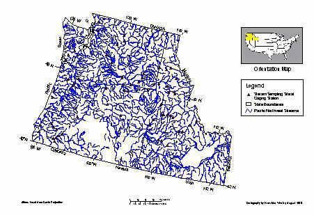
The study area includes 71 designated salmon habitat recovery streams in the Pacific Northwest, including Oregon, Idaho, and Washington (Figure 1). Castro (1997) has determined geomorphic indicators at the reach scale of these streams. The hydrologic modeling and land use assessment was conducted at the watershed scale.
Figure 1: Study Area.
DATABASES
The primary databases compiled for this study include (1) a United States Geological Survey (USGS) gaging station database, (2) a LULC database for the Pacific Northwest, and (3) one degree DEMs for the entire study area. Other coverages utilized include Hydrologic Unit Coverages (HUC), and Digital Line Graphs of streams in the United States, both provided by the USGS as Background Data Sets for Water Resources. HUC are hydrologic areas based on surface topography that contain the drainage area of major rivers and surface drainage basins. HUC units at the fourth level, the most detailed level of classification available, were utilized for this study. This study further utilized state outline coverages for Oregon, Washington, and Idaho.
METHODOLOGY
The topography and relief of an area determine the flow of surface water. ArcView Spatial Analyst provides hydrologic modeling functions that use the DEM’s surface values to model the flow of surface water. ArcView Spatial Analyst Hydrologic Modeling extension, in conjunction with supplemental methods, was utilized for watershed delineation for 71 stream sampling points. The following methodology focuses on (1) the acquisition and manipulation of DEMs; (2) the determination of pour points and the delineation of watersheds; and (3) quality control and spatial editing of the delineated watersheds.
1. DEM Acquisition and Manipulation
Ninety-seven one degree DEMs were downloaded in compressed format from the USGS web sites for Oregon, Washington, and Idaho, and were converted to grids. The grids have a scale of 1:250,000, which are consistent with the scale of the LULC data layer. USGS DEM grids are in the geographic projection system (ground units: arc-seconds, surface units: meters). Hydrologic modeling was conducted using the original projection system. All delineated watersheds required conversion to Albers Conic Equal Area projection system after hydrologic modeling was completed.
DEMs were mosaiced for the entire study area to allow for accurate delineation of watersheds extending over grid boundaries. The Grid Transformation Tools extension for Spatial Analyst hosts the mosaic function for grids.
Hydrologic modeling was conducted on DEM grid mosaics for the Pacific Northwest. The following hydrologic modeling functions were utilized for DEM manipulation: FillSinks, FlowDirection, and FlowAccumulation. These hydrologic modeling functions use the mosaiced DEMs as input grids, model the surface characteristics, and create new grids. The new grid output files were then used to model watershed characteristics.
The hydrologic modeling function FillSinks ‘corrects’ the DEM grid through identifying any sinks in the original DEM grid. Sinks are incorrect values on the DEM that are of lower elevation compared to all surrounding values. Water flowing into sinks would not be able to flow out and therefore cause inaccuracies in flow path and drainage mapping as well as in watershed delineation. The FillSinks request fills these artificial depressions and creates a new grid. The new output filled grid created served as the base grid for all following hydrologic modeling.
The FlowDirection function was utilized to determine the directions to which water would flow out of each cell. The filled grid was used as the input grid for the FlowDirection request. The FlowDirection function created a new output grid (Figure 2).
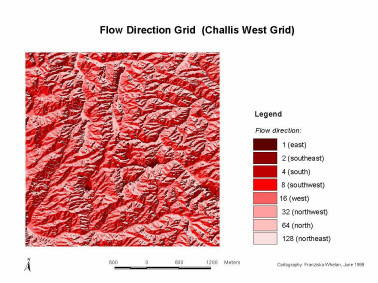
Figure 2: Flow Direction Grid.
The hydrologic modeling function FlowAccumulation was used to create a stream network. The FlowAccumulation function calculates the number of upslope cells flowing into a location based on the flow direction grid. The flow accumulation grid displays the major drainage network (Figure 3).
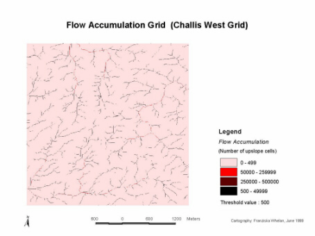
Figure 3: Flow Accumulation Grid.
Data processing and management issues need to be considered when working with large mosaiced grid files. The largest mosaiced grids in terms of data size were produced from the FlowAccumulation function, averaging 150 MB per state and over 500 MB for the entire Pacific Northwest. Hardware available to the user will determine if modeling is possible at the state or regional scale. During the initial phase of the project, a PC with 333 MHz with 128 MB RAM was used and was incapable of calculating the FillSinks, FlowDirection, FlowAccumulation, and FlowPath requests on mosaics of DEM grids for the individual states or the entire Pacific Northwest. During the later phase of the project, a PC with 433 MHz with 128 MB RAM was utilized and capable of executing these requests on large mosaics. Mosaics are required if watersheds extend over several individual grids. Also, working with mosaics saves time. All hydrologic modeling functions need to take place on the original mosaiced DEM. Watersheds will not accurately delineate if grids are mosaiced after the various hydrologic functions were executed on the individual grids.
A stream station database including 71 USGS gaging stations along designated salmon habitat recovery streams in the Pacific Northwest was compiled for this study. Streams were selected based on watersheds that contain critical habitat for salmonids. The selected stream gages monitor watersheds ranging from approximately 11,000 acres to 5 million acres in size.
Before watershed delineation, the exact location of each gaging station had to be determined. Latitude and longitude data allowed for an approximate location of stream stations. However, for correct watershed delineation, it is crucial to locate the stream sampling point on the stream. Minor deviations from the stream or flow path would initiate the delineation of small side watersheds rather than the target watersheds.
The digital stream sampling point layer indicated the approximate location of stream stations. USGS gage station location maps, available through the USGS water data web site at scales of 1:12,808, 1:25,617, 1:51,234, 1:102,468, and 1:205,265 were utilized as supplemental information. Hard copy topographic maps at scales of 1:150,000, and 1:300,000 for Oregon (DeLorme, 1996), 1:150,000 for Washington (DeLorme, 1998), and 1:250,000 for Idaho (DeLorme, 1998), as well as selected USGS topographic maps at scales of 1:250,000 were referenced to determine the exact location for each stream sampling point.
Once the location of the stream sampling point was determined, the pour point had to be placed exactly onto the stream network, or onto the flow path. Flow path delineation utilized the filled grid, FlowDirection grid, and FlowAccumulation grid. Hydrologic properties need to be set to define the correct input FlowDirection and FlowAccumulation grids. The filled grid should be the active grid in the view. The filled grid allowed for good visualization of the topography in the area.
The flow accumulation layer displays the stream network. Flow paths of medium-sized and large streams overlay the stream network defined by the FlowAccumulation grid. The view of the FlowAccumulation grid was manipulated through changing the value and label in the legend editor (legend type: graduated color, color ramps: red monochromatic). The stream network was clearly displayed when the value and label of the first legend entry, which was the entry with the smallest value range and lightest color, was changed to a value range of 1-500. This change caused values of 500 and larger to be displayed in dark colors. The stream network was then clearly displayed in dark colors and black on a light colored background. Classifying values by their standard deviations and displaying the first category in a light color and the following categories in dark colors also displayed the stream network well.
Once the pour point was defined, the watershed request was used to delineate the watershed based on that pour point. Since the described methodology allowed for accurate determination of stream sampling points, the WatershedTool Script for watershed delineation was modified (script see Appendix A). By default, the WatershedTool script uses a snap distance of 240 cells around the pour point for watershed delineation. Delineated watersheds would therefore include cells that are downstream or at level of the actual watershed. The snap distance of 240 cells was designed by the Environmental Systems Research Institute (Esri) with the assumption that pour points could not be located accurately on the grid. However, since the described methodology allowed for accurate pour point location, the default 240 cell snap distance would introduce an unnecessary error to the watershed delineation. Therefore, the grid cell accumulation value for a snapped pour point was changed from 240 to 0 cells in the following script line:
‘calc watershed
theWater – theFlowDir.Watershed(theScrGrid.SnapPourPoint(theAccum,0))
Watershed delineation was now based on the determined pour point only. The snap distance was 0. This script change caused a significant increase in delineation accuracy. Users should only change the script if the exact location of the pour point has been determined.
Delineated watersheds
are displayed in the view as temporary grids called ‘a watershed’ and need to be converted to shapefiles. The DEM delineated watersheds were in the geographic projection system (Figure 4). A conversion from the geographic projection system to Albers Conic Equal Area projection system was conducted to allow for future overlays with the LULC data. ArcInfo was utilized for this conversion, since ArcView does not offer a projection conversion for the geographic projection having arc-seconds as ground units and meters as surface units.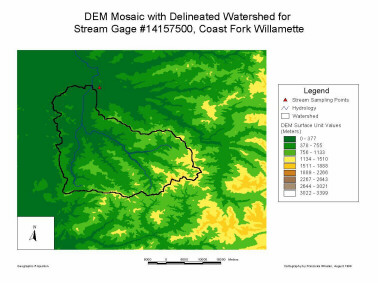
3. Quality Control and Spatial Editing
To determine the accuracy of the digitally delineated watersheds, quality control was conducted that included reference checks using a digital stream layer, the LULC data layer and topographic maps, flow path comparison, HUC references, and area check. The delineated watersheds were compared to features displayed on these reference maps and coverages.
Land features of concern included reservoirs that could potentially alter the flow paths on the DEMs and therefore contribute to incorrect watershed delineation. When large bodies of water or reservoirs were located within or upstream of the delineated watersheds, flow path delineation was conducted to check for potential flow path interruption or reversion. The corresponding original watersheds in the geographic projection system and the filled grid, FlowDirection grid, and FlowAccumulation grids were used for this check.
The LULC layer and the digital stream layer were used to confirm the location of land use features, including streams, lakes, reservoirs, urban areas, and roads, within or outside of the delineated watersheds. Topographic maps were referenced to confirm the location of these land features relative to the delineated watershed boundaries.
Quality control was also conducted through area comparisons for all watersheds. A database of USGS determined drainage areas for stream gaging stations was compiled and used as a control for all watersheds. USGS drainage areas were determined through manual watershed delineation on 1:24,000 USGS topographic maps. USGS drainage areas are listed for all gaging stations on the individual gaging station’s web site. Areas of the digitally delineated watersheds were calculated after the conversion of all watersheds to Albers Conic Equal Area projection system. A merged shapefile containing all delineated watersheds was created to allow for an efficient area calculation using the table of that merged shapefile. Watershed areas were calculated using the calculator function and the request [shape].Returnarea/(4046.95*640). The units of the Albers Equal Area projection system were set in meters. Dividing the area by (4046.95*640) converts the area to square miles. Differences between USGS defined areas and delineated watersheds were determined in both absolute and relative values (square miles and percent).
Watersheds were re-delineated, when watershed areas exceeded set difference limits from the USGS reference areas. The process of re-delineation revealed the underlying problems causing inaccurate delineation. Following successful re-delineation, all quality control checks were conducted again. When re-delineation confirmed delineation problems due to faulty DEM grids or other watershed characteristics, supplemental methods including HUC and digitizing were utilized to correct or adjust the delineated areas.
HUC was referenced when area differences were detected for relatively medium and large area watersheds. HUC was used to identify missing sub-watersheds for delineated watersheds that were too small compared to the USGS drainage area. For watersheds larger than the USGS reference value, HUC were referenced to identify areas that should not have been included in the delineated watersheds. Small area differences were eliminated by spatially editing the boundaries of the digitally delineated watersheds to correspond with HUC boundaries.
ANALYSIS
Statistical methods used to determine the reliability of Spatial Analyst Hydrologic Modeling extension for watershed delineation included t-tests, ANOVA F-tests, and descriptive statistics. The evaluation of the described methodology is based on one degree DEMs used for this study. Spatial Analyst Hydrologic Modeling may perform at different levels of accuracy with different data sets.
1. Suitability of Spatial Analyst Hydrologic Modeling for Watershed Delineation
A two-sample t-test for means was used to determine whether Spatial Analyst Hydrologic Modeling extension was suitable for watershed delineation with no supplemental methods used. Accuracy of the initially delineated watersheds using Spatial Analyst was determined through comparing watershed areas of the digitally delineated watersheds to USGS defined drainage areas. Statistically, there is no significant difference (two-sided p-value = 0.63) for watersheds delineated using Spatial Analyst Hydrologic Modeling as the only method and USGS reference areas (Table 1).
The data set did not include ten watersheds that were delineated using topographic maps and hydrologic units only. These ten watersheds could not be delineated using Spatial Analyst Hydrologic Modeling due to watershed pour points located in areas of no gradient, or watersheds located in metropolitan areas. The one degree DEMs were unsuitable for watershed delineation in dense urban areas because of human altered topography and hydrologic features.
|
Initial Delineated Area (square miles) |
USGS Reference Area (square miles) |
|
|
Mean |
971.147541 |
949.142623 |
|
Variance |
1903047.295 |
1969923.307 |
|
Observations |
61 |
61 |
|
Hypothesized Mean Difference |
0 |
|
|
df |
60 |
|
|
t Stat |
0.473161147 |
|
|
P(T<=t) two-tail |
0.637815141 |
|
Table 1: Two-sample t-test for Watersheds Delineated Using Spatial Analyst Hydrologic Modeling and USGS Reference Areas.
Despite no significant difference for a group of 61 watersheds, area differences were quite large for some individual watersheds. Table 2 lists the ten maximum area differences for watersheds delineated using Spatial Analyst Hydrologic Modeling as the only method compared to USGS reference areas. The mean initial difference for 61 delineated watersheds was 229 square miles with a standard deviation of 1288 square miles. Area differences varied from 0 square miles up to 2,679 square miles.
|
Gage Number |
Initially Delineated Area (square miles) |
USGS Reference Area (square miles) |
Initial Difference (square miles) |
Initial Difference (%) |
|
13235000 |
3135 |
456 |
2679 |
588 |
|
14359000 |
1486 |
2053 |
567 |
28 |
|
14048000 |
7106 |
7580 |
474 |
6 |
|
12027500 |
574 |
895 |
321 |
36 |
|
12205000 |
360 |
105 |
255 |
243 |
|
14033500 |
2107 |
2290 |
183 |
8 |
|
14207500 |
601 |
706 |
105 |
15 |
|
12031000 |
1201 |
1294 |
93 |
7 |
|
12414900 |
365 |
275 |
90 |
33 |
|
13336500 |
1825 |
1910 |
85 |
4 |
Table 2: Ten Maximum Area Differences for Initially Delineated Watersheds Using Spatial Analyst Hydrologic Modeling as the Only Method Compared to USGS Reference Areas.
Due to the large area differences for some individual watersheds, difference limits were arbitrarily set despite the statistical insignificant difference between the two groups. Difference limits were set to be > 4%, or >10 square miles. Watersheds exceeding area difference limits were re-delineated or corrected using the supplemental methods described. Spatial editing was applied to 46 out of 61 delineated watersheds.
Six outlier watersheds exceeded the difference limits (Table 3). These watersheds were initially spatially edited, however the final delineated watershed areas still exceeded the set difference limits. Based on referenced topographic maps these six watersheds were judged accurate and repeated spatial editing was avoided since this could lead to data manipulation in terms of ‘matching’ the data with the required target areas. For example, one outlier watershed exceeded the limit for the 4% area difference. The exceptionally small watershed was initially delineated with an area of 25 square miles, spatial editing was applied and resulted in a final watershed area of 20 square miles. A two square mile difference amounted to 12.9%, compared to the USGS reference area of 17.7 square miles. The other five outlier watersheds exceeded the square mile difference limit, however, due to the extremely large size of these watersheds, deviations from the USGS reference areas amounted to less than 2% of the total watershed area.
|
Gage Number |
Initially Delineated Area (square miles) |
USGS Reference Area (square miles) |
Initial Difference (%) / (SQ MILES) |
Final Difference (%) / (sq miles) |
|
13346800 |
25 |
18 |
41 / 7 |
13 / 2 |
|
13296500 |
791 |
802 |
1 / 11 |
2 / 15 |
|
13302005 |
834 |
845 |
1 / 11 |
1 / 11 |
|
14312000 |
1657 |
1670 |
1 / 13 |
0.7 / 13 |
|
13333000 |
3297 |
3275 |
1 / 22 |
0.5 / 16 |
|
13266000 |
1382 |
1460 |
5 / 78 |
1 / 17 |
Table 3: Outlier Watersheds that Exceed Area Difference Limits.
Watershed accuracy improved after applying spatial editing and supplemental methods, including reference checks using a digital stream layer, the LULC data layer, topographic maps, and HUC references. Figure 5 illustrates the increase in delineation accuracy. Drainage areas of watersheds delineated using Spatial Analyst as the only method was compared to final delineated watersheds and USGS reference areas.
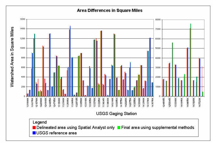
Figure 5: Area Differences in Square Miles After Initial and Final Watershed Delineation Compared to USGS Reference Areas.
2. The Influence of Watershed Attributes on Watershed Delineation Using Spatial Analyst Hydrologic Modeling
Watershed attributes that influenced delineation accuracy of Spatial Analyst hydrologic modeled watersheds were specific to one degree DEM data. Watershed attributes of concern included large metropolitan areas, and little or no gradients. Other watershed attributes that may influence watershed delineation accuracy include drainage area, and land use features, including reservoirs or lakes. Delineation problems due to the above became evident immediately for ten watersheds. These ten problem watersheds were delineated through digitizing or through correlation with established Hydrologic Units. These watersheds were not included in the following analysis, since delineation problems were not caused by the malfunctioning of the software but by data problems.
Watershed delineation using the Spatial Analyst Hydrologic Modeling extension was impossible for watersheds with large metropolitan areas. This study included the following three mainly metropolitan watersheds; USGS gaging stations 14202000 (Pudding River at Aurora), 14203500 (Tualatin River near Dilley), and 14207500 (Tualatin River near West Linn). Delineation attempts resulted in nonsensical shapefiles of several grid cells in one long row and were not remotely suitable for statistical testing. These watersheds were manually delineated using 1:250,000 USGS topographic maps and digitized.
Watershed pour points with little to no gradient also influenced delineation accuracy. Faulty delineations were immediately evident for these extreme cases. Watersheds with little or no gradient were also digitized after manual watershed delineation on 1:250,000 USGS topographic maps. Some of these watersheds were identical to the metropolitan watersheds.
Watershed delineation using Spatial Analyst Hydrologic Modeling may be inaccurate when lakes or reservoirs are located within or near watersheds. Occasionally, reservoirs and lakes were inaccurately delineated as a watershed boundary. To avoid these types of inaccuracies, topographic maps and LULC coverages were referenced for quality control.
Two-sample t-tests assuming unequal variances were conducted to determine if delineated drainage area was correlated to specific delineation methods. Watersheds delineated using HUC as a supplemental method were significantly larger than watersheds successfully delineated using Spatial Analyst Hydrologic Modeling only (t-test, two-sided p-value < 0.05). This difference is partly accountable to the relatively small scale of the fourth order HUC data. There is suggestive but inconclusive evidence that digitized watersheds were smaller than watersheds that were delineated using Spatial Analyst Hydrologic Modeling only (t-test, two-sided p-value = 0.09). The sample set for the digitized watersheds also includes the smallest watershed (18 square miles) of this study. Mean area for watersheds delineated using HUC as a supplemental method was 1,868 square miles, compared to a mean watershed size of 878 square miles for watersheds successfully delineated with Spatial Analyst Hydrologic Modeling only, and a mean drainage area of 429 square miles for delineated watersheds supplemented by digitizing.
3. Supplemental Methods Required to Improve Delineation Accuracy
Supplemental spatial editing was required for 46 of 61 watersheds exceeding the defined difference limits. HUC data, topographic maps, and LULC were utilized as reference data layers for all spatial editing.
One-way ANOVA F-tests were conducted to determine whether the differences between final delineated area and USGS reference area were significantly different for different supplemental delineation methods. Delineation differences relative to watershed size (differences in %) differed significantly for the different supplemental methods (one-way ANOVA F-test, two-sided p-value < 0.01), however, no significant difference was determined for absolute area differences (differences in square miles). Mean final area difference for Spatial Analyst delineated watersheds was 1.2% (Standard Error 0.1%), with a maximum difference of 3.8%. Mean difference for delineated watersheds supplemented by digitizing was 4.1% (Standard Error 3.0%), including one outlier of 12.9%. Mean area difference for watersheds supplemented by HUC was 0.7% (Standard Error 0.3%) with a maximum difference of 1.6%. The tested data set only included the 61 watersheds that were initially delineated with Spatial Analyst Hydrologic Modeling. The ten problem watersheds mentioned earlier were not included, since the initial watershed area could not be delineated using Spatial Analyst Hydrologic Modeling. The initially Spatial Analyst delineated areas were compared to the final areas improved through supplemental methods.
A two-sample t-test was conducted to determine whether area differences between delineated watershed areas and USGS reference areas were reduced by utilizing the supplemental methods described. There is moderate but inconclusive evidence for a decrease in differences from the initially delineated watersheds using Spatial Analyst Hydrologic Modeling only and the final delineated watersheds (two-sided t-test, p-value = 0.07). Supplemental methods increased the accuracy of watershed delineation. Initially, watershed areas differed 19%, or 89 square miles, from their reference areas before the utilization of supplemental methods. Mean area differences were reduced to only 1%, or 5 square miles, after supplemental methods were used. There is no significant difference in the increase in area accuracy (two-sample t-test, two-sided p-value > 0.05) between the supplemental methods used.
CONCLUSION
This study successfully developed and evaluated an integrated methodology for watershed delineation relying on the Spatial Analyst Hydrologic Modeling extension. This study does not present a cookbook for watershed delineation, since successful watershed delineation is a case by case study. Project planning is a crucial component of GIS based hydrologic research. Proper identification of appropriate data layers and initial data preparation before any modeling is conducted is often overlooked. Development and evaluation of the described methodology was based on one degree DEM data. Spatial Analyst Hydrologic Modeling may perform at different levels of accuracy with different DEM data sets.
Successful watershed delineation requires accurate determination of pour point location. Pour points can be accurately located by referencing supplemental large scale topographic maps displaying the pour point in combination with DEM flow path delineation. Accurate pour point location will allow the user to edit the WatershedTool script in ArcView by reducing the grid cell accumulation value for a snapped pour point from 240 to 0. The edited script increases watershed area and boundary accuracy.
Initial watershed areas delineated using Spatial Analyst only and USGS reference watershed areas were not significantly different (two sided p-value = 0.63). Despite no significant difference, numerous watersheds had quite large area differences, ranging up to 2,679 square miles. (This data set of 61 watersheds did not include ten watersheds with characteristics unsuitable for automated delineation.) Approximately 75% of the watersheds in this study required supplemental spatial editing based on set difference limits. Regardless of area difference, boundary checks are recommended for all watersheds as a quality assurance measure.
Spatial Analyst hydrologic delineation supplemented by accepted delineation methods, such as hydrologic unit maps and manual digitizing of topographic maps, provided the most accurate watersheds. The utilization of specific supplemental methods is a case by case study based on watershed characteristics, including watershed size, land use, and large hydrologic features. Typically, hydrologic units were the stronger reference for relative large watersheds (> 1,800 sq. miles). Watershed features, such as little to no gradient or dense urban areas surrounding the pour point, had the strongest negative impacts on delineation. To a lesser degree, delineation problems caused by lakes and reservoirs were often overcome by referencing topographic and LULC maps.
Spatial Analyst Hydrologic Modeling is suitable for watershed delineation when quality control is conducted. Recommended quality control steps include reference checks using a digital stream layer, a LULC data layer, and topographic maps, flow path comparison, HUC references, and area check. This study recommends to consistently employ these quality control steps.
The described methodology provides a basis for suture studies that intend to utilize Spatial Analyst Hydrologic Modeling for hydrologic, geomorphic, or other watershed related research. This method represents one solution among a spectrum of possible solutions to the mapping and delineation of watersheds. Traditional solutions include hand delineation and manual digitizing. Spatial Analyst Hydrologic Modeling extension was chosen primarily for its efficiency and objectivity of watershed delineation, and for an ease of digital mapping and later spatial analysis or overlays with other data. Recommended future research includes an analysis of watershed delineation accuracy using Spatial Analyst Hydrologic Modeling for DEMs with higher resolution.
In addition to its primary objective of developing and evaluating a methodology for digital watershed delineation, this study has compiled a land use and cover map for the entire Pacific Northwest. Beyond watershed related applications, this information might also serve as an important component in the study and management of many other natural resources in the Pacific Northwest and comparable landscapes.
APPENDIX
APPENDIX A: Watershed Delineation Script With Changed Value For Pour Point Snap Distance
Watershed delineation utilizes the aGrid.Watershed request, which determines the contributing area above a set of cells in a Grid. The total area flowing to a given pour point is the output of the aGridWatershed request. The pour point is the lowest point along the watershed boundary. Therefore, the DEM should be free of artificial sinks. The following script was used for this study. The defualt value of 240 cells for the snap-to-pour-point-distance was changed to 0 cells.
' WatershedTool script
av.UseWaitCursor
theView = av.GetActiveDoc
theDisplay = theView.' 3D.AddToTIN
theView = av.GetActiveDoc
thePrj = theView.GetProjection
' get the surface
theSurfaceTheme = theView.GetEditableTheme
if (theSurfaceTheme = NIL) then
return NIL
end
theTin = theSurfaceTheme.GetSurface
' Get collection of feature themes to pass to tin builder dialog
themeList = {}
for each t in theView.GetActiveThemes
if (t.Is(FTheme)) then
theFTab = t.GetFTab
if (theFTab.GetShapeClass.IsSubclassOf(Point) or
(theFTab.GetShapeClass.IsSubclassOf(MultiPoint) and (theFTab.GetShapeClass.GetClassName <> "MultiPatch"))) then
themeList.Add(t)
end
end
end
tinBuildList = tinBuilderDialog.Show(themeList)
if (tinBuildList.Count = 0) then
return NIL
end
' call TinBuilder script to do work
success = av.Run("3D.TinBuilder",{theTin,tinBuildList,TRUE,"Add Features to TIN",thePrj})
if (success.Not) then
MsgBox.Error("Error adding features to" ++ theSurfaceTheme.GetName + ".","Add Features to TIN")
return NIL
end
theSurfaceTheme.Invalidate(TRUE)GetDisplay
theGridTheme = theView.GetActiveThemes.Get(0)
p = theDisplay.ReturnUserPoint
theGrid = theGridTheme.GetGrid
mPoint = MultiPoint.Make({p})
theSrcGrid = theGrid.ExtractByPoints(mPoint, Prj.MakeNull, FALSE)
' get flow dir and acc from extension preferences
hydroExt = Extension.Find("Hydrologic Modeling (sample)")
if (hydroExt = NIL) then
MsgBox.Error("Cannot find extension!","Watershed Tool")
return NIL
end
flowDirGThemeName = hydroExt.GetPreferences.Get("Flow Direction Property")
theFlowDirGTheme = theView.FindTheme(flowDirGThemeName)
if (theFlowDirGTheme = NIL) then
MsgBox.Error("Cannot find flow direction theme in view!","Watershed Tool")
return NIL
end
theFlowDir = theFlowDirGTheme.GetGrid
flowAccGThemeName = hydroExt.GetPreferences.Get("Flow Accumulation Property")
theFlowAccGTheme = theView.FindTheme(flowAccGThemeName)
if (theFlowAccGTheme = NIL) then
MsgBox.Error("Cannot find flow accumulation theme in view!","Watershed Tool")
return NIL
end
theAccum = theFlowAccGTheme.GetGrid
' calc watershed
theWater = theFlowDir.Watershed(theSrcGrid.SnapPourPoint(theAccum,0))
' rename data set
aFN = av.GetProject.GetWorkDir.MakeTmp("watt", "")
theWater.Rename(aFN)
' check if output is ok
if (theWater.HasError) then return NIL end
' create a theme
gthm = GTheme.Make(theWater)
' set name of theme
gthm.SetName("A Watershed")
' add theme to the specifiedView
theView.AddTheme(gthm)
REFERENCES
Anderson, J.R., E.E. Hardy, J.T. Roach, and R.E. Witmer. 1976. A Land Use and Cover Classification System for Use With Remote Sensor Data. U.S. Geological Survey Professional Paper 964.
Castro, J. 1997. Bankfull Flow Recurrence Intervals: Patterns in the Pacific Northwest. (submitted to) Water Resources Research.
Delorme. 1996. Oregon Atlas and Gazetteer. 2nd ed. Freeport, ME.
Delorme. 1998. Idaho Atlas and Gazetteer. 2nd ed. Yarmouth, ME.
Delorme. 1998. Washington Atlas and Gazetteer. 4th ed. Yarmouth, ME.
DOI, USGS. 1991. Land Use and Land Cover and Associated Maps Factsheet. U.S. Geological Survey, Reston, VA.
DOI, USGS. 1986. Land Use Land Cover Digital Data from 1:250,000 and 1:100,000-Scale Maps Data User Guide 4. U.S. Geological Survey, Reston, VA.
Environmental Systems Research Institute. 1996. Advanced Spatial Analysis Using Raster and Vector Data. Using the ArcView Spatial Analyst. Redlands, CA.
Fels, J.E., and K.C. Matson. 1998. A Cognitively-Based Approach for Hydrogeomorphic Land Classification Using Digital Terrain Models. 1998 Esri User Conference Proceedings. Environmental Systems Research Institute, Redlands, CA.
Gordon, N.D., T.A. McMahon, and B.L. Finlayson. 1994. Stream Hydrology. An Introduction for Ecologists. John Wiley & Sons, New York.
Guttenberg, A.Z. 1965. New Directions in Land Use Classification. Urbane, IL: Bureau of Community Planning, University of Illinois.
Horton, R.E. 1932. Drainage Basin Characteristics. Transactions of the American Geophysical Union 13:350-361.
Johnston, C.A., N.E. Detenbeck, J.P. Bonde, and G.J. Niemi. 1988. Geographic Information Systems for Cumulative Impact Analysis. Photogrammetric Engineering and Remote Sensing 54(11):1609-1615.
Kilpatrick, F.A., and H.H. Barnes. 1964. Channel Geometry of Piedmont Streams as Related to Frequency Floods. U.S. Geological Survey Professional Paper 422-E.
Kompare, T.N. 1998. A Preliminary Study of Near-Stream Vegetative Cover and In-Stream Biological Integrity in the Lower Fox River, Illinois. 1998 Esri User Conference Proceedings. Environmental Systems Research Institute, Redlands, CA.
Leopold, L.B., and T.Maddock. 1953. The Hydraulic Geometry of Stream Channels and Some Physiographic Implications. U.S. Geological Survey Professional Paper 252. 57 p.
Leopold, L.B. 1996. A View of the River. Harvard University Press, Cambridge, MA.
Leopold, L.B., M.G. Wolman, and J.D. Miller. 1964. Fluvial Processes in Geomorphology, Freeman, San Francisco, 522p.
Loelkes, G. L. Jr., G.E. Howard, Jr., E.L. Schwertz, Jr., P.D. Lampert, and S.W. Miller. 1983. Land Use/Land Cover and Environmental Photointerpretation Keys. U.S. Geological Survey, Reston VA.
Mitchell, W. B., Guptill, S. C., Anderson, K. E., Fegeas, R. G., and C.A. Hallam. 1977. GIRAS--A Geographic Information and Analysis System for Handling Land Use and Land Cover Data. U.S. Geological Survey, Professional Paper 1059, p 16, Reston, VA.
Osborne, L.L., and M.J. Wiley. 1988. Empirical Relationships Between Land Use/Cover and Stream Water Quality in an Agricultural Watershed. Journal of Environmental Management 26:9-27.
Richards, K. 1982. Rivers, Form and Processes in Alluvial Channels. Methuen, 358pp.
Strahler, A.N. 1957. Quantitative Analysis of Watershed Geomorphology. Transactions of the American Geophysical Union 38:913-920.
U.S. Environmental Protection Agency. 1999. Geographic Information Retrieval Analysis System (GIRAS) Directory.
ftp://ftp.epa.gov/pub/spdata/EPAGIRAS.U.S. Geological Survey. 1990. Land Use and Land Cover Digital Data From 1:250,000- and 1:100,000-Scale Maps--Data Users Guide 4. Reston, Virginia.
U.S. Geological Survey. 1999. USGS – Water Resources of the United States: Background Data Sets for Water Resources: HUC and Streams (Digital Line Graphs). http://water.usgs.gov/GIS/background.html
U.S. Geological Survey. 1999. Land Use / Land Cover Data (1:250,000). http://edcwww.cr.usgs.gov/glis/hyper/guide/1_250_lulcfig/states.html
U.S. Geological Survey. 1999. Global Land Information System (GLIS): 1-Degree-Digital Elevation Models.
http://edcwww.cr.usgs.gov/glis/hyper/guide/1_dgr_demfig/states.htmlU.S. Geological Survey. 1999. United Staes Water Resources Page: National Water Information System (NWIS). http//waterdata.usgs.gov/nwis-w.
Youberg, A.D., D.P. Guertin, and G.L. Ball. 1998. Developing Stream-Watershed Relationships for Selecting Reference Site Characteristics Using ARC/INFO. 1998 Esri User Conference. Environmental Systems Research Institute, Redlands, CA.
Franziska Whelan
PhD Candidate
Department of Geosciences
Oregon State University
Mailing Address:
68-697 A Crozier Dr.
Waialua, HI 96791
808 637-4250 (V)
whelann@aol.com