Helen Purves and Carol Doering

Wolves and People: Assessing cumulative impacts of human disturbance on wolves in Jasper National Park

Abstract

Jasper National Park is using an Arc/Info Geographic Information System to model cumulative effects of human disturbance on wolf habitat effectiveness and movement patterns. The models accommodate "what if" scenarios, enabling investigation of land use management alternatives. The Graphic User Interface provides a user-friendly environment. The models have the flexibility of overriding default parameters, allowing the user to address changes in expert knowledge, or to transfer the models to other study areas.

Introduction

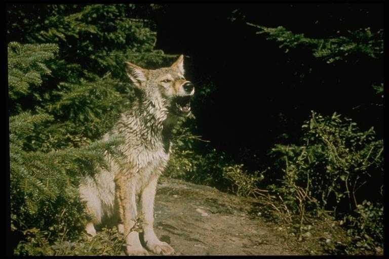
Wolves (Canis lupus) are one of the key indicator species for the cumulative effect assessment of humans on the landscape in Jasper National Park (JNP), (Figure 1). In the central Canadian Rockies, the most suitable habitat for 366 vertebrates occurs within the primary range of gray wolves (Paquet et al 1996), who show a strong affinity for low elevation valley bottoms. In many North American areas, this species has been extirpated or alienated in areas of high human use activity (Harris 1984). The mechanisms of this displacement are often not clear, but include intolerance of humans or direct mortality due to hunting and other control actions (Weaver et al. 1986). Avoidance of human activities by wildlife has become an important consideration in habitat and wildlife management.

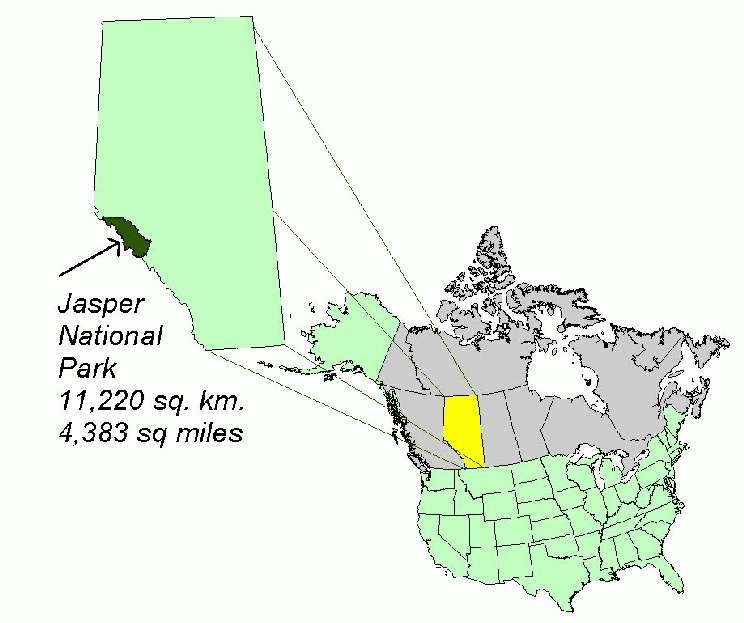
Figure 1. Location of Jasper National Park.

Human activity within JNP may be causing adverse cumulative environmental effects. More than 1.8 million people visit the park annually (Kjvoren, 1999 : personal communication ). As human activity in a natural area increases, cumulative environmental effects can result from individually minor yet collectively significant uses, occurring over space and time (Weaver et al. 1986). Human activities such as hiking, camping, driving or simply human presence may cause ecosystem-wide impacts. Cumulative Effects Assessment (CEA) analyzes the effects of human activities on a system and whether or not those effects exceed or fall short of thresholds necessary for the maintenance of a given indicator.

The wolf study area (Figure 2) is located roughly at the center of JNP, in the montane ecoregion. This ecoregion is of high importance to both wildlife and humans, comprising only 7% of the park's area. Within the study area, three river valleys intersect, creating a zone of convergence for wildlife movement and dispersal called the Three Valley Confluence (TVC). The majority of the park accommodation and amenities supporting the tourism industry, the town, and infrastructure for trans-Canada rail, highway, and pipeline transportation industries, also converge in this area. Other landscape disturbances include high use trails, gravel extraction sites and former landfills.

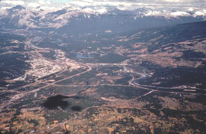
Figure 2. Three Valley Confluence study area

Banff National Park, just to the south of Jasper National Park developed the Wolf Habitat Effectiveness Model (Paquet et al 1996). They used univariate and multivariate statistical tests to assess the relationship of 1,248 wolf telemetry points to the physical environment and human activities. Last winter, Jasper National Park used the research conducted in Banff to develop a GIS based application to assess the effects of humans on wolf behaviour and ecology within the Three Valley Confluence area of JNP. The model assesses which habitats are inherently attractive to these species and how that attraction is modified by the presence of humans.

Objectives and steps to complete the wolf cumulative effects assessment tool.

The primary objective of this modeling exercise is to quantify the observed effects of human developments on wolf habitat and wolf movement patterns. An Arc/Info Geographic Information System (GIS) was used to create two applications. The first was a Wolf Cumulative Effects Assessment (CEA) tool, for modeling potential wolf habitat, without human use, and for modeling realized habitat, accounting for human use. The second model was a least-cost path model for validating the wolf CEA model and to help identify important travel corridors.

The steps involved in this project:

1. Model wolf potential habitat/movement patterns with no human use for both winter and summer;
2. Model wolf realized habitat/movement patterns accounting for human use;
3. Validate and refine the models by using least-cost path analysis, and wolf tracking sessions. Use the least-cost path application to identify travel corridors;
4. Compare potential and realized habitat (habitat loss, fragmentation, increases in cost of movement).

Potential wolf habitat/movement patterns under "pristine conditions".

It is generally assumed that wolf habitat preference is strongly related to availability of prey (Holroyd and Van Tighem 1983, Huggard 1991); ease of travel (Cowan 1947, Mech 1970, Peek 1991, Paquet et al. 1992); and location of den sites and rendezvous areas (Mech 1970). Wolves in the Canadian Rockies show strong affinity for low elevation valleys (Paquet et al 1996).

This model uses four components to calculate the potential wolf habitat (Figure 3). The components are:6 availability of prey, slope, aspect and elevation. They were all assigned eigenvector weights, based on their importance when calculating potential wolf habitat, Table 2. The eigenvector weights came form the multivariate analysis of 1,248 telemetry points in the Canadian Rockies (Paquet et al. 1996). The user can change the default weightings and probabilities through the GUI interface.

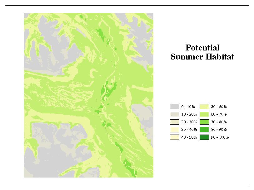
Figure 3. Potential Habitat Map

Table 2. Weighting of potential habitat components.

The composite Potential Habitat Model (PHM) is a combination of the standardized individual components, using the formula:

PH = (PA*W_PA)+(S*W_S )+(A*W_A)+(E*W_E)

Where: PH= Potential Habitat for wolves

PA = Prey availability for wolves

S = Slope

A = Aspect

E = Elevation

W = Eigen-vector weights

Elevation

Elevation was divided into two classes. Areas of the park below 2000 m had a 95% probability and those above 2000m had a 5% probability. The elevation cutoff can be changed for summer and winter. The 2000m is the default but this can be changed by the user.

Aspect

Aspect was divided into 8 classes at 45°intervals and a last class for flat terrain Table 3.

Table 3. Default aspect probabilities.

Prey availability

Jasper National Park has an ecological land classification (ELC) that integrates landform, soil and vegetation information (Holland and Coen 1982). About 124 ecosites (unique soil and vegetative associations) are recognized and mapped at 1:50,000 scale (about 35 ha).

The prey abundance layer is calculated for both summer and winter. The species used to calculate prey abundance ratings are elk, moose, deer, mountain sheep, caribou, and beaver. Beaver was only used in the summer. The ELC was converted to a grid and each cell had a habitat rating for each of the prey species, nil (0.0), very low (0.2), low (0.4), medium (0.6), high (0.8) and very high (1.0). Each prey species was then weighted (Table 4) based on their abundance.

Table 4. Default prey weightings

The habitat rating for each species was multiplied by the weighting and the six species added together.

PA=(HS_elk*W_elk)+(HS_moose*W_moose)+(HS_deer*W_deer)+(HS_sheep*W_sheep)+(HS_caribou*W_caribou)~

+(HS_beaver*W_beaver)

Where: PA = Prey availability for Wolves

HS = Habitat Suitability

W = Weighting

If an ecosite was rated very high for all six species, the best possible rating it would attain is 1.0, conversely the worst is 0.0.

Slope

PWe used the following equation to map probability of wolf occurrence relative to slope in degrees Y=28.18405*.931377^X. The data was log transformed and smoothed. This reduced the sensitivity of the model to extreme slope values, and increased the sensitivity to changes in the lower ranged values. This results in a surface where the highest probability of occurrence is 28.18405.

Realized wolf habitat once human use is considered.

Human activities are often concentrated in prime wildlife habitat. Thus, avoidance of human activities by wildlife has become an important consideration in habitat and wildlife management.

The disturbance component for the effectiveness model uses human activity mapping done for previous ecosystem studies. The point, line and polygon data are assigned a human use intensity value for the summer (August) and winter (February). Human use was categorized into seven classes on an exponential scale based on park visitation records and expert knowledge.

The human use features are broken down into activity groups containing combinations of motorized or non-motorized types of activity and high or low intensity of activity (more or less than 1,000 disturbance events per month by default). Each activity group is assigned a disturbance coefficient and zone of influence. Default values are used, however, the user can change these defaults through the GUI interface. The zone of influence (buffer) identifies the area in which wolves will be disturbed by the activity and the disturbance coefficient identifies the degree of disturbance within the zone of influence. Disturbance coefficients are rated on a scale of 0 to 1 based on how wolves would respond to a given activity. A disturbance coefficient of 0 implies total displacement. A disturbance coefficient of 1 implies no displacement.

Some human use features are attractants to wolves in the winter. A few of the low use trails, where the snow gets packed down by human activity, create an attractant to the wolves. They find it easier to travel along a packed trail rather than travelling through the deep snow. The application allows the user to apply special coefficients (>1.0) to those features which we know are attractants to wolves.

For this model disturbance coefficients from the Banff National Park are adopted for the types and intensities of human use (Paquet, personal communications January 28,1999). The model uses these values as defaults. However, the values may be edited interactively, through the GUI interface. The special coefficients may also be assigned through the GUI interface.

The human activity layer is buffered using the Arc/Info regions feature type to accommodate overlapping disturbances. The cumulative disturbance coefficient for a given polygon is a product of the individual overlapping disturbances.

This product represents a polygon's cumulative disturbance coefficient (CD) and is calculated using the equation

CD_p = Dc_pai * Dc_paj *Dc_pak....DC_pax

Where:

CD_p represents the cumulative disturbance for the polygon

Dc_pai..DC_pax represents the disturbance coefficents for each region in which the polygon

exists

The potential habitat value is then combined with the cumulative disturbance coefficient to calculate the realized ability of wolves to continue using the habitat component. For every polygon realized habitat (RHp) was calculated using the equation

RHp = PHp *CDp.

Where:

RHp = Realized Habitat for the polygon

PHp = Potential Habitat for the polygon

CDp = Cumulative Disturbance for the polygon

A polygon with a realized habitat rating of 0 is interpreted as containing no value to wolves, a polygon with a rating of 1 is interpreted as the best possible habitat (Figure 4).

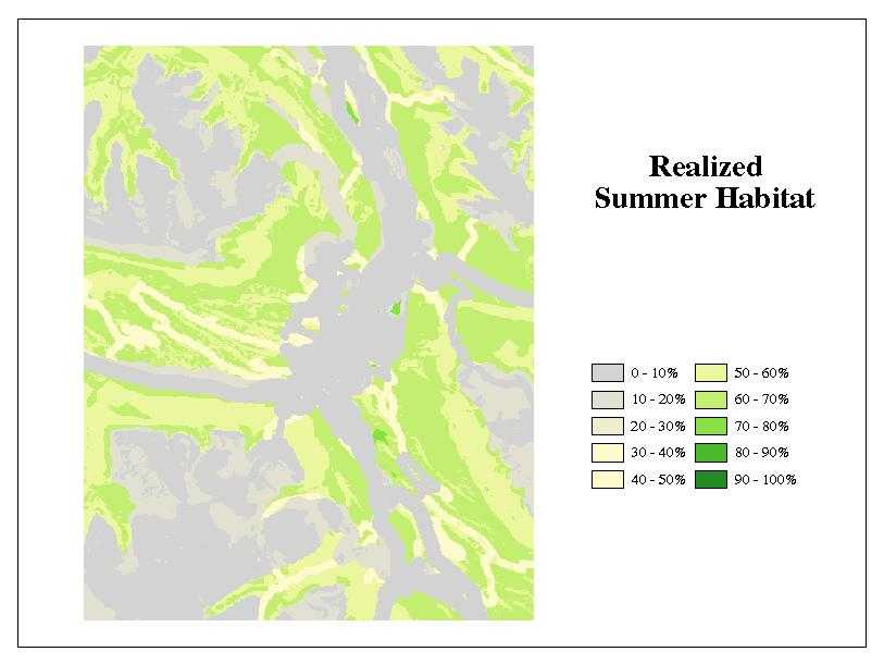
Figure 4. Realized Habitat Map

Model validation and corridor identification through least-cost path analysis.

Two methods were used to validate the models. First, GPS tracking session were overlaid on the prey, slope, aspect, and elevation data. Second, a least-cost path application was developed to predict the least-cost paths between start and end points. The predicted paths were then compared to the actual tracking session. The least-cost application was also used to identify important travel corridors.

During the winter of 1998-1999, researchers tracked wolves with a GPS. They collected over 105 kilometres of data. Tracking session data, along with the start and end points, were imported into the GIS. The tracking sessions were converted to GRID.

The wolf habitat effectiveness model was validated by overlaying tracking sessions on the prey, slope, aspect and elevation data, and measuring the distance to the closest human use feature (Figure 5). The results were then compared to the original potential habitat equations to look for areas to improve.

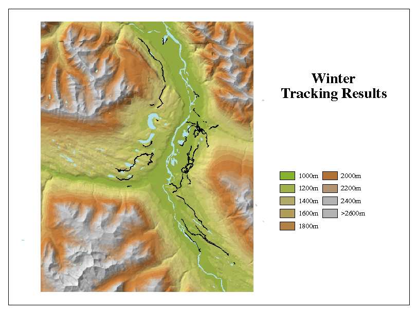
Figure 5. Tracking sessions overlaid on elevation

A least-cost path application was developed to test for accuracy of the model as well as for identifying travel corridors. We assume the least-cost path, offers a wolf the greatest probability of survival in traversing the entire distance. This was facilitated by Arc/Info GRID functions costdistance and costpath, but it is also biologically based. Although an animal may not chose the least-cost (optimum) path, if it did it would encounter fewer hazards or obstacles, would spend less time in traveling, and would travel thought habitat with higher probability of containing food, thus increasing its probability of survival. The least-cost path balances prey availability, ease of movement, minimum euclidean distance and degree of "connectivity" between the two endpoints (Walker, Craighead, 1997).

A second method of validating the models was to use the least-cost path application to calculate predicted paths, and then compare the predicted and actual paths both statistically and visually (Figure 6). The predicted least-cost path and the actual paths were overlaid on prey, slope, aspect and elevation. We will do statistical t-tests to compare the two paths. The final comparison is a visual check to look at the differences between the predicted and actual paths.

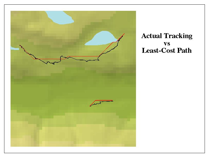
Figure 6. Comparison of a predicted least-cost path and actual tracking sessions.

The identification of travel corridors is a very important component of the least-cost path application. We will use 500 random start and end points and have the computer generate the least-cost paths between all of them. The least-cost paths will then be added together and viewed. Wherever there are multiple least-cost paths overlapping it is assumed that area is of importance to wolves. We would also like to use the corridor command to identify travel corridors through the TVC.

The least-cost path application is a valuable tool in validating the model, as well as in identifying travel corridors through the TVC.

Habitat effectiveness: the comparison of potential habitat and realized habitat.

Habitat effectiveness was determined by comparing potential and realized habitat for habitat loss, fragmentation and increases in cost of movement.

To measure habitat loss and fragmentation we grouped the final potential (PH) and realized (RH) habitat values into four habitat quality types by applying an equal interval reclassification scheme. We will then run it through the ArcView FragStat extension available from the Lakehead University web page http://flash.lakeheadu.ca/~rrempel/patch/.

Patch Analyst is an extension to the ArcView GIS system that facilitates the spatial analysis of landscape patches. There are two versions of the program, the full version, which analyses both polygon and grid data structures, and the Vector Edition (VE), which analyses only polygon data. The full edition requires the Spatial Analyst extension, and this version works with ArcView shapefiles and grids, and ArcInfo coverages and grids.

Some 28 patch metrics are calculated, and these include mean and median patch size, patch size coefficient of variance, edge density, mean shape index, fractal dimension, interspersion and juxtaposition, Shannon's diversity indeces, and core area index. The program can also create a new shape with patch metric attributes attached. Summary statistics are reported at either the patch or landscape scale. The various patch metrics follow the definitions in fragstats (McGaril and Marks 1993).

Angus Carr programmed the extension through funding from the Sustainable Forest Management Network (NCE) and with support from the Centre for Northern Forest Ecosystem Research. Patch Analyst© is not public domain, but may be used free of charge under an attached license agreement.

To measure the increase in cost of movement, we will convert tracking sessions GRID and overlay them on the reciprocal of the potential and realized habitat coverages. We will then compare the cost of moving along the tracking session with no human influence (potential habitat) to the cost of moving along the same track with the influence of humans (realized habitat).

GUI interface

The GUI interface for the wolf cumulative effects application allows the user to interactively set the output workspace; input coverages; retrieve and edit coefficients and model parameters; edit the human use attribute values; run the models and print the results in report and map formats. The interface for the least-cost path application allows the user to set the output workspace, input coverages, set the output data names and set the cell size. The interfaces keeps track of all of the model inputs in a status report (Figure 7.). The status report is displayed at all times.

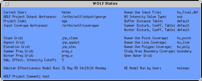
Figure 7. The status report

There are seven steps involved in running the wolf cumulative effects assessment model.

1. Set the output workspace. This workspace can be an existing or newly created.
2. Set a three letter run code. Each run of the model requires a three-letter code (unique to the output workspace), which is associated with that particular run. All of the results from the models such as coverages, maps and reports are prefixed with this three letter code and stored in the output workspace.
3. Set the input coverages. The interface allows users to select the input coverages for the three models. The coverages required to run the model may be seen in Table 1.
4. Set the model parameters. The human use attributes, buffer distances and disturbance coefficient files are chosen. The user may also change the default parameters, such as aspect breakdown, elevation cut off, and weighting coefficients (Figure 8). This allows the models to be enhanced with future research and validation, as well as making them adaptable to different geographic regions. The model parameters are printed in the summary reports.
5. Edit the human use type and intensity if required. If an area appears to be a blockage to wolf movement, the user can run a "what if" scenario by altering the human use feature attributes, and then run the model again to see what type of gain or loss has to be realized.
6. Run the model.
7. Create, view and print maps and reports. The maps and reports have all been standardized. The application allows the user to create poster output for the three models in both French and English.

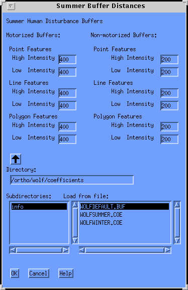
Figure 8. Disturbance coefficients selection and editing window

There are six steps involved in running the least-cost path model

1. Set the output workspace. This can be an existing or newly created workspace.
2. Set the input coverages. The user is asked to set the start, and end points of the tracking sessions, the tracking sessions and the friction layer (The potential or realized habitat from the wolf model).
3. Set the name of the output file.
4. Change the cell size if you wish. The default is 50m.
5. Run the model.
6. Create, view and print maps and reports.

Both applications also contain tools for coverage and info table maintenance. These tools allow the user to move, copy or kill coverages and info tables. They also allow the user to view info tables, coverages and grids. This is useful for checking input and output coverages or grids.

Summary

Cumulative effect assessment is a key component for managing landuse in JNP. The wolf CEA application along with the least-cost path application developed by the park, provides park managers, planners and wildlife specialists with the necessary tools to make better management decisions. The ability to perform "what if" scenarios provides the users with a valuable tool to help predict the results of various management options.

The two applications were designed for use by front line managers, rather than GIS staff. It expands upon wolf modeling work previously completed in other jurisdictions by providing a relatively simple GUI interface. It also helps to enforce model integrity through the tracking of data inputs and model parameters. In addition, the flexibility of overriding model default parameters provides the ability to adjust the models to address changes in expert knowledge and parameters for other jurisdictions.

Acknowledgments

Jasper National Park would like to thank Carol Doering and the staff at The Forestry Corp. for coding these models. Adrian Walton, a volunteer student, has spent the past two months working with the models and doing the analysis of results, his work is greatly appreciated by the park. We would also like to thank Paul Paquet for his help in adapting his models for Banff National Park to Jasper National Park. Thanks also to Dr. Roger Tomlinson for his guidance while implementing our GIS.

Literature cited