Michael R. Kunzmann, Royden J. Hobbs, Cynthia S. A. Wallace, and Stuart E. Marsh
________________________________________________________________________
AVHRR Imagery Analysis and Habitat Modeling as Planning Tools for Conducting Yellow-billed Cuckoo (Coccyzus americanus occidentalis) Surveys in Arizona.
________________________________________________________________________


ABSTRACT:


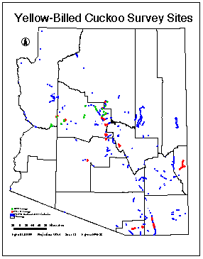
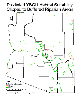
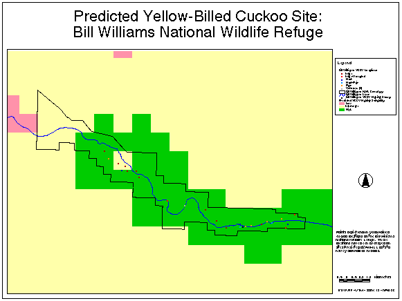
The western yellow-billed cuckoo, Coccyzus americanus occidentalis, typically nests in mature riparian forests and woodlands along central and southern Arizona drainages and locally along the Virgin river. Riparian habitat alteration from vegetation clearing, stream diversion, water management, agriculture, urbanization, overgrazing, and recreation have caused reductions in the breeding range of the yellow-billed cuckoo over the last 60 years (Laymon and Halterman 1987). As a result, western yellow-billed cuckoos have been petitioned for possible listing under the Endangered Species Act (1973 as amended). To facilitate current species censusing and monitoring activities, a GIS and concomitant correlation models are relied upon to delineate potential yellow-billed cuckoo habitat and to help determine cost effective field data collection strategies. Initially, GIS and modeling efforts were constrained to legacy data sets such as existing layers of environmental data and historic breeding locations of western yellow-billed cuckoos in Arizona. Eventually, these course scaled methods for identifying potential locations of yellow-billed cuckoo breeding habitats will be refined to include higher resolution spatial data and a wider array of secondary database attributes required to succinctly define habitat requirements.


Introduction

  In 1993, the yellow-billed cuckoo was split into two subspecies C. a. americanus (the eastern subspecies) and C. a. occidentalis (the western subspecies)(Franzreb and Laymon 1993). The western yellow-billed cuckoo (Coccyzus americanus occidentalis) has been in decline for the past 60 years throughout the western United States. The decline is reportedly due to habitat destruction (Franzreb 1987), decreased water tables (Phillips et al. 1964), and possibly the use of pesticides (Gaines and Laymon 1984, Laymon and Halterman 1986b, Rosenberg et al. 1991). In February of 1998, 23 groups filed a petition with the United States Fish and Wildlife Service (USFWS) seeking endangered species status for the western subspecies of the yellow-billed cuckoo. The USFWS typically has one year, unless an extension is granted, to decide if species listing is warranted.


Historically, the western yellow-billed cuckoo occupied and bred in riparian zones from southern British Columbia to northern Mexico, including the states of Oregon, Washington, southwestern Idaho, California, Nevada, Utah, western Colorado, Arizona, New Mexico, and western Texas. Current evidence suggests that western yellow-billed cuckoo breeding is now restricted to California, Arizona, New Mexico, Utah, extreme western Texas, Sonora, Chihuahua, and south irregularly to Zacatecas, Mexico (Howell and Webb 1995, Russell and Monson 1998). The largest breeding populations of the Western yellow-billed cuckoo (Coccyzus americanus occidentalis) in the United States may now be confined to New Mexico and southeastern Arizona. Population estimates of the yellow-billed cuckoo include; less than 50 pairs in California (Halterman 1991); an estimated 902 pairs in the middle Rio Grande and the Pecos rivers in New Mexico (Howe 1986); and an estimated 846 pairs along the major rivers of southern Arizona (Groschupf 1987). The exact distribution and habitat requirements of the western yellow-billed cuckoo in Arizona are not known. Preliminary surveys in 1998 were conducted in areas where the species was historically noted. The yellow-billed cuckoo has been associated with cottonwood-willow dominated broadleaf deciduous riparian habitat (Hamilton and Hamilton 1965, Gaines 1974, Gaines and Laymon 1984, Laymon and Halterman 1986a, Halterman 1991). The purpose of this one year preliminary project was to revisit historic locations for site fidelity by confirming the presence and absence of yellow-billed cuckoo records, to collect and better delineate vegetation characteristics in presumably predictable yellow-billed cuckoo habitat, and to utilize AVHRR remote-sensing satellite imagery processing techniques to predict potential bird habitat.


Yellow-billed Cuckoo Survey Techniques

  California census protocols for this species (Laymon 1998) were modified by a team of experts under Arizona State Game and Fish Department leadership. Numerous project cooperators, including the Arizona State Game and Fish Department, the USGS BRD Colorado Plateau Field Station, and numerous private-sector organizations and individuals, have been instrumental in collecting presence and absence data.   Site surveys were conducted using a "look-see" approach as described by Bibby et al. (1992). With the "look-see" method, potential sites are identified before surveys are started. The method relies on prior knowledge of historic habitats, possible habitat preferences, expert opinion, and knowledge of the basic ecology of the species. This approach allowed project cooperators to delineate surveying sites (apriori) on USGS topographical maps or aerial photographs. All 1998 sites visited were eventually digitized and incorporated into ARCINFO for subsequent analysis (Figure 1). Global Positioning System (GPS) receivers and background maps from ungenerated ARCINFO coverages, when used in conjunction with Geolink GPS data collection software, were extremely valuable in helping us find difficult survey sites on back-county roads. In addition, Geolink was critical in delineating the shape and size of yellow-billed cuckoo habitat patches (polygons) in the field.


Historic Cuckoo Locations Surveyed in 1998
Figure 1: Point locations represent historical yellow-billed cuckoo sites visited by survey teams in 1998. The background polygons show the potential distribution of yellow-billed cuckoo habitat as predicted by the Arizona Gap Analysis Program. To locate and census the birds, surveyors used a playback recording of the paired cuckoo's contact call ("Kowlp" call) to elicit a response from nearby yellow-billed cuckoos (Laymon 1998). Johnson et al. (1981) recommended this technique when surveying for secretive bird species or species that occupy dense vegetation. Recordings were played every 100 m (328 ft) to detect (attract) yellow-billed cuckoos. If no cuckoos were detected during the initial listening period, the tape was played for five complete calls with a one minute delay between call playbacks. In some cases, we did not need to solicit a yellow-billed cuckoo call because the birds were calling when we arrived at the site or during the setup of our vegetation transects. Most bird surveys were conducted between June 15 to August 20 to coincide with the peak of the yellow-billed cuckoo's breeding season in Arizona (Hamilton and Hamilton 1965, Nolan and Thompson 1975).   Vegetation Field Techniques   All methods for recognizing and defining plant communities are methods of classification. The objective of classification is to group together a set of individuals on the basis of their attributes (floristics: presence/absence/abundance, physiognomics: morphology/life-form/size). The final result of classification is a set of similarly grouped plant communities based on one or more attributes. The methods for carrying out vegetation classification and analysis are many and varied. Because of budget limitations, the one-year duration of the project, and the lack of knowledge about what set of vegetation attributes are preferred by yellow-billed cuckoos, we decided to use three different field techniques to characterize the vegetation communities found at each habitat patch. The techniques selected were: (1) a modified Braun-Blanquet approach using dimensionless releve's and prominence rankings (Warren 1982, Bennett et al. 1998), (2) a quantitative sampling method using systematic circular plots to record detailed species composition, canopy-based measurements, percent cover, and other vegetation characteristics, and (3) a simple method of counting all 5.0 cm diameter-at-breast-height trees at least 2.0 m in height. Whenever feasible, paired 50 m x 30 m quadrats (separated by 50m plus a single-digit random offset) were established adjacent to stream corridors to examine riparian community variability. All three field methods were utilized on every vegetation quadrat for comparative and analytical purposes. An effort was made to select vegetation quadrats that would "best" typify the vegetation at each yellow-billed cuckoo site. Vegetation measurements, such as tree and shrub canopy volumes, are easily visualized after the raw data is entered into a database (Figure 2). Field data will be used to calculate similarity coefficients and matrices to help examine the relationships between sites with and without birds. In addition, site vegetation characteristics will be used as "training" sets for calibrating satellite-based imagery classification techniques.


Vegetation Parameters Represented in Graphical Form
Figure 2: Results of vegetation data collected from circular plots on a 50 m x 30 m transect grid. Maroon and blue cylinders represent canopy volumes of trees and shrubs, respectively. Yellow cylinders represent the maximum height of vegetation in a plot.


The locations of all quadrat origins were determined by GPS and transect lines for circular plots were laid out by magnetic compass bearings to within 3 degrees. Early examination of the vegetation data collected to date seems to indicate that the field methodologies are sensitive enough to delineate differences in riparian vegetation communities that change as a function of the perpendicular distance from the primary stream course. For example, in southeastern Arizona Typha latifolia/Baccharis salicifolia strands are integral with the active stream channel. These hydroriparian communities may be followed by mesoriparian, "middle-aged", 10-20 year-old Salix gooddingii/Sambucus mexicana vegetation associations which help to stabilize and define the river channels. A third major community type consisting of a more mature 40-60 year-old Populus fremontii/Celtis recticulata associations may also exist with a more open understory (Figure 3). Typically within the drainage the vegetative species composition of the habitat will vary according to the last major disturbance event and numerous site historical factors including a variety of anthropogenic factors.


Vegetation Parameters Represented in Graphical Form
Figure 3: The San Pedro river is characteristic of southern Arizona habitat for the yellow-billed cuckoo. The vegetation community changes from a  Typha latifolia/Baccharis salicifolia strand to a Populus fremontii/Celtis recticulata association as a function of distance from the river.  

Preliminary GIS Analysis

  Prior to summer field work a GIS database was developed to facilitate project planning, to digitally delineate historic habitat patches, and to characterize habitat patches by examining polygon size, shape, elevation, and other GIS related variables. For example, site ownership and access were determined to evaluate the necessity of conducting yellow-billed cuckoo surveys on non-public lands which would require access permits and authorization from individual land owners (Table 1). We also used "habitat polygons" as input for our preliminary imagery-based AVHRR analysis of potential yellow-billed cuckoo habitat. Individual GPS positions of birds and expert delineation of historic habitat polygons served as the primary sampling unit for the purposes of habitat prediction. Polygons were also required to obtain legacy riparian vegetation information so a stratified-random sample of potential habitats could be determined in advance that would include all possible vegetation community types. Arizona has a predicted 797,876 hectares of yellow-billed cuckoo habitat, that represents approximately 2.7 % of the total land area in Arizona.


Ownership of Yellow-billed Cuckoo Habitat in Arizona
Table 1: Land ownership of yellow-billed cuckoo habitat predicted by the Arizona Gap Analysis Program was examined to determine the necessity of conducting yellow-billed cuckoo surveys on private lands.


Image Processing Techniques and Preliminary Habitat Predictions   In this preliminary analysis, we evaluated the temporal dynamics of yellow-billed cuckoo areas as a function of the temporal change in vegetation spectral signatures obtained from satellite imagery. Changes in vegetation communities (dynamics) are related to features of the landscape such as vegetation phenology and condition. The imagery/data used in this study was collected by the National Oceanic and Atmospheric Administration's (NOAA) Advanced Very High Resolution Radiometer (AVHRR) satellite (EDC 1994, Eidenshink 1992). The relatively coarse spatial resolution of the sensor (each image pixel is equivalent to a 1km2 area on the ground) is offset by its high temporal resolution.


AVHRR images are acquired daily, as opposed to the bi-weekly revisit cycle of many other sensors. AVHRR data are often used in research on land-cover change since the frequency of data availability permits the detection of short-lived vegetation and landscape changes that may be missed by other sensors. A derived image reflecting vegetation photosynthetic activity, the Normalized Difference Vegetation Index (NDVI) is calculated as a maximum value composite for every 2-week period to produce a cloud free image. The NDVI is calculated from the reflectance values of the visible and near-infrared regions of the electromagnetic spectrum and is sensitive to various biophysical vegetation characteristics, such as biomass and percent cover (Price 1992, Huete and Jackson 1987). (Visit the Arizona Regional Information Archive (ARIA) to view a movie of the 26 2-week NDVI composites of Arizona during 1998, http://aria.arizona.edu). The movie shows areas of abundant vegetation in bright green and areas of little or no vegetation in red. The loop starts in January and ends in December, showing the timing and progression of vegetation green-up across the state. We applied various mathematical techniques (described below) to extract measures describing the temporal dynamics of the NDVI signal at each pixel.

  The first objective of this study was to use satellite imagery to create a potential yellow-billed cuckoo habitat map. To do this, we identified quantifiable relationships between the broad-scale, high-temporal resolution AVHRR imagery and cuckoo habitat patches (polygons) and or individual point sightings from 1998 yellow-billed cuckoo surveys. Image pixels containing either expert-defined habitat patches or actual cuckoo sightings were examined for distinctive temporal attributes. We hypothesized that:


The GIS software packages utilized for this type of analysis were Environmental Systems Research Institute (Esri) ArcView 3.1 and Arc Info 7.1.2. Image processing was accomplished in Erdas Imagine 8.3.1. Data preprocessing of the original data and the creation of the fourier-derived matrices were accomplished using MathWorks Matlab 5.2. Additional data processing was conducted using Microsoft Excel 97. Statistical analyses were performed in the Statistical Product and Service Solutions (SPSS) 8.0 software package. Results were exported to Excel for the creation of representative graphs. Using these tools, we performed the following:


    1. We compiled four sets of point data:
      1. The 1998 data with positive bird responses (data set A)
      2. The 1998 data with negative bird responses (data set B).
      3. Points sampled from polygons representing expert-defined cuckoo habitat patches (data set C). These points were generated in Arc/Info by first converting the polygon coverage to a 120 meter grid. The grid was then converted to a point coverage, resulting in a point sample of the habitat patches weighted by the size of each patch.
      4. Points sampled from polygons of perennial riparian areas (data set D). The riparian coverage was also converted to a point coverage after conversion to a 120-meter grid. A random sample of 5000 points was selected from the original 43,000-plus points for analysis. Of these 5000 points, 181 points fell outside the polygon of the state of Arizona due to the coarseness of the derived grid and were eliminated, resulting in a final coverage of 4819 points.
       
    2. We layer-stacked the 26 AVHRR NDVI bi-weekly composite images for 1998 and extracted the temporal NDVI profile for all image pixels in the state of Arizona. New images representing summary measures of these profiles were created in Erdas Imagine as follows:
      1. The average of the 26 points defining the pixel profiles: AZ98_TSAVE.
      2. The standard deviation of the pixel profiles: AZ98_TSSDE.
      3. The coefficient of variation of the pixel profiles: AZ98_COV.
       
    3. We calculated the multi-temporal Standardized Principal Components (SPCA) for the 26-layer image of the state of Arizona for 1998 using Erdas Imagine and extracted Principal Components 1, 2, and 3 as three new images (AZ98_PC1, AZ98_PC2, and AZ98_PC3). For long-time series of AVHRR bi-weekly NDVI composites, the first principal component (PC1) represents the characteristic NDVI, and can be shown to be equivalent to the average NDVI for the time period analyzed. The second principal component (PC2) is found to represent "seasonality," and the extremes of PC2 correspond to landscapes with summer green-up and those with winter green-up (Eastman and Fulk 1993, Hirosawa et al. 1996). The meaning of the third principal component (PC3) is less clear, but inspection of eigenvector loadings suggest to us that it may represent a "spring-fall" seasonality analogous to the PC2.
    4.  

    5. We imported the 26-layer image into Matlab as a three-dimensional matrix and performed a Fourier analysis of the temporal NDVI profiles at each pixel. Four new images were created as follows:
      1. The "Direct Current" (DC) component, which is the best fit of a flat line to the profile (AZ98_DC).
      2. The magnitude of the first frequency component, which is the amplitude of the single sine wave that fits the annual profile best (AZ98_MAG).
      3. The phase of the first frequency component, which is the position of the peak (between -pi and +pi) of the single sine wave that fits the annual profile best (AZ98_PHASE).
      4. To facilitate interpretation, the phase data were also rescaled to represent the Julian date (0 to 365) of the sine wave peak (AZ98_JULIAN).
       
    6. We joined all the point data (sightings, habitat patches, and random riparian) to the 10 derived images in ArcView. This produced 10 values at each sample point representing the values of the respective derived images at the location of each point. Each of these values can be thought of as an index of the temporal dynamics of the landscape, and represent the following general types of measures:
    7. Amount of greenness:

      1. AZ98_TSAVE Time series average
      2. AZ98_PC1 Principal component 1
      3. AZ98_DC Fourier direct current
      Timing of the green-up:
      1. AZ98_PHASE Fourier phase
      2. AZ98_JULIAN Fourier phase (rescaled)
      3. AZ98_PC2 Principal component 2
      4. AZ98_PC3 Principal component 3
      Variability of the greenness:
      1. AZ98_TSSDE Time series standard dev.
      2. AZ98_COV Time series COV
      3. AZ98_MAG Fourier magnitude
  Using SPSS software, we performed two-tailed Student's t-tests for independent means to compare the following sets of data (Table 2):
      1. Sightings with birds (set A) vs. Random riparian points (set D)
      2. Habitat patch points (set C) vs. Random riparian points (set D)
      3. Sightings with birds (set A) vs. Sightings without birds (set B)


sets A vs. D Sets C vs. D sets A vs. B
alpha
diff.
Alpha
diff.
alpha
diff.
AZ98_TSAVE
++
neg
++
neg
++
neg
AZ98_TSSDE
++
neg
++
neg
AZ98_COV
+
neg
++
pos
AZ98_DC
++
neg
++
neg
++
neg
AZ98_MAG
++
neg
++
pos
AZ98_JULIAN
++
pos(8)
++
neg(34)
AZ98_PC1
++
neg
++
neg
+
neg
AZ98_PC2
++
pos
++
pos
AZ98_PC3
++
neg
++ = Significant at the 0.05 level, + = significant at the 0.10 level
 
 
Table 2: Results of a Students t-test to compare data sets, as follows: Data set A = Sightings with birds; Data set B = Sightings without birds; Data set C = Points sampling cuckoo habitat patches; Data set D = Points randomly sampling riparian areas. The alpha value shows whether the two data sets are significantly different at either the 90% confidence level (+) or at the 95% confidence level (++). The "diff." value shows the direction of the value difference between the sets, with the magnitude shown parenthetically for significant difference in the Julian date. For example, we see that the riparian areas posses a generally higher average NDVI value than either the sightings with birds or the cuckoo habitat patches, since the AZ98_TSAVE t-test result is significant at the 95% confidence level with a negative difference for sets A vs. D and sets C vs. D.  
These early results can be summarized as follows:   An issue of concern with these data sets is that the sightings data possess few points. There are only 39 sightings with birds and 25 sightings without birds. For this reason, and because t-test results revealed similar relationships between cuckoo habitat and sightings with birds, we chose to select the habitat variables based on the results of the t-tests between the cuckoo habitat points and the riparian points. Based on these results, all variables except PC2 can be used to discriminate between general riparian areas and cuckoo habitat. These variables were selected for evaluation as inputs to the final habitat model   Habitat Preference Class Creation   The derived images of the selected variables were stratified into cuckoo preference classes based on their observed distribution. A three-tiered preference class was created using the standard deviation of the data set to partition the data. Any data up to 1 standard deviation away from the mean was ranked Highly Preferred; data from 1 to 2 standard deviations away was considered Moderately Preferred, and anything outside of 2 standard deviations was considered Not Preferred.   The data ranges specified were then used to create maps of preferred habitat for each variable. The resulting maps were further evaluated using the actual sightings data. The number of cuckoo sightings for each of the three preference categories (Highly Preferred, Moderately Preferred and Not Preferred) were tallied and the results are shown in Table 3.
 
Preference
AZ98_TSAVE
AZ98_TSSD
AZ98_COV
AZ98_MAG
AZ98_PROD
AZ98_JULIAN
AZ98_PC3
AZ98_PC1
Low
1
0
0
0
1
0
1
2
Medium
13
20
13
9
10
15
6
34
High
25
19
26
30
28
24
32
3
Total Birds
39
39
39
39
39
39
39
39
 
Table 3: Number of birds sighted in each category for each variable.
 
The indices of temporal dynamics that best predict the locations of cuckoo sightings were used in the final model. These are shown in bold in Table 3 and include two measures each describing the Amount, Timing and Variability of greenness, as follows: Amount of greenness:
  1. Time Series Average NDVI (AZ98_TSAVE)
  2. Fourier "DC" Productivity (AZ98_PROD )
Timing of the green-up:
  1. Fourier Phase, rescaled (AZ98_JULIAN)
  2. Standardized Principal Component 3 (AZ98_PC3)
Variability of the greenness:
  1. Coefficient of Variation (AZ98_COV)
  2. Fourier Magnitude (AZ98_MAG)
 
To create the habitat model, the six preference maps were reclassified to numerical labels representing the relative quantity of sightings within the categories, such that "Rare or Not Preferred" = 1 , "Uncommon or Somewhat Preferred" = 2 , and "Common or Preferred" = 3. The habitat model was then created by simply adding together the six stratified data layers. This produced a single model for preferred habitat with 13 classes, ranging in value from 6 ('Not Preferred' on all input layers) to 18 ('Preferred' on all input layers). Figure 4 shows the results of the habitat model for the whole state. However, because yellow-billed cuckoo's are primarily found in riparian habitats the final surface generated was clipped (limited) to perennial streams with a 500 m buffer (Figure 5).  
Figure 4:  Statewide prediction of yellow-billed cuckoo habitat using AVHRR data.


Figure 5: AVHRR predicted yellow-billed cuckoo habitat clipped to perennial water courses buffered to 500m.
 
Preliminary Conclusions   A commonly used, rigorous test of a model's effectiveness involves first withholding a subset of the total data points from inclusion in the model. The model is 'trained' on the remaining set of data, and is then used to predict the excluded points. The amount of error seen in the real versus predicted data is an indication of the model's reliability. The ultimate test of the current model will occur when additional cuckoo sightings are obtained from this year. If the model is able to predict this year's cuckoo locations (presence and absence), its functionality will be supported. An example of the potential usefulness of these techniques is data recently collected from the Bill Williams National Wildlife Refuge where actual nesting locations appear to be in fairly good agreement with the habitat prediction model (Figure 6). However, these results are very preliminary and may not be applicable to other locations around Arizona.


Bill William's River Data Overlayed on Predicted Yellow-billed Cuckoo Habitat
Figure 6: AVHRR predicted yellow-billed cuckoo habitat overlayed with known yellow-billed cuckoo locations  on the Bill Williams National Wildlife Refuge.  


A number of factors influencing the number of birds counted in a sampling unit (mapping plots, polygons, transects or parts of transects, unequal temporal and spatial resolution sampling factors, inherent habitat variability, weather factors, and a wide array of human errors), may introduce a large amount of error. Consequently, using simple presence/absence bird counts and polygons delineated by a combination of historical factors and local experts as inputs for a yellow-billed cuckoo distribution and habitat model may lack precision if not accuracy. Unfortunately with limited time and funding, statistical extrapolation is a necessity if not a requirement for intelligent decision making by land managers and conservation experts. Models are valuable tools but all population estimates based on extrapolations should be carefully interpreted (Dawson 1981).

  Acknowledgements   We would like to thank the USGS Biological Resources Division Regional Office and staff for project funding to do the field work necessary to conduct this preliminary investigation; Dr. William Halvorson, Unit Leader, USGS BRD Sonoran Desert Field Station at the University of Arizona for his dedicated support of graduate students, field assessment activities, and the necessary disk drives to store the data; Dr. Charles Van Riper, Unit Leader, USGS BRD Colorado Plateau Field Station, Flagstaff, and his staff for census work, data sharing, and digitizing efforts; Mr. Robert MaGill, Arizona Game and Fish Department for project coordination; Ms. Murrelet Halterman for her practical advice and yellow-billed cuckoo expertise; The School of Renewable Natural Resources and the following Staff members and graduate students who assisted with the project and related field work: Mr. Peter Bennett, Mr. Alexander Rybak, Ms. Patty Guertin, and Mr. Volodymyr Ivakhnyk; We also thank Mr. Douglas Richardson of Baker-GeoResearch Inc. (Billings, Montana) for his support and the educational use of Geolink mapping software to train a new generation of students on GPS technologies; Ms. Jessica Walker for her assistance with the image processing; and Dr. Lee Graham for her compilation of the Arizona Gap Analysis yellow-billed cuckoo habitat model.   REFERENCES CITED   Bennett, P., M. Kunzmann, W. Halvorson. 1998. Manual for the GAP program: collecting vegetation classification data. USGS BRD Cooperative Park Studies Unit. The University of Arizona, Tucson, AZ. Unpublished.

Bibby, C.J., N.D. Burgess and D.A. Hill. 1992. Bird census techniques. Academic Press. New York, NY. 257 pp.

Dawson, D.G. 1981. Experimental design when counting birds. Studies in Avian Biology No. 6:392-398.

Eastman, J.R. and M. Fulk (1993) Long Sequence Time Series Evaluation Using Standardized Principal Components. Photogrammetric Engineering and Remote Sensing. 59(6):991-996.

EDC (1994) Conterminous United States AVHRR Data on CD ROM - User's Manual, U.S. Department of Interior, Eros Data Center, Souix Falls, SD.

Eidenshink, J. C. (1992) The 1990 Conterminous U.S. AVHRR Data Set. Photogrammetric Engineering and Remote Sensing. 58:809-813.

Franzreb K., and Laymon, S.A. 1993. A reassessment of the taxonomic status of the yellow-billed cuckoo. Western birds 24:17-28

Franzreb, K. 1987. Perspectives on managing riparian ecosystems for endangered bird species. Western birds 18:10-13.

Gaines D.A. and S.A. Laymon. 1984. Decline status and preservation of the yellow-billed cuckoo in California. Western Birds 15:49-80.

Gaines, D. 1974. Review of the status of the yellow-billed cuckoo in California: Sacramento Valley Populations. Condor 76:204-209.

Groschupf, K. 1987. Status of the yellow-billed cuckoo (Coccyzus americanus occidentalis) in Arizona and New Mexico. Contract No. 20181-86-00731.

Halterman M. 1991. Distribution and habitat use of the yellow-billed cuckoo (Coccyzus americanus occidentalis) on the Sacramento River, California, 1987-1990. MS Thesis, California State University, Chico.

Hamilton W.J. and M.E. Hamilton. 1965. Breeding characteristics of yellow-billed cuckoos in Arizona. Pages 405-432 in Proceedings of the California Academy of Sciences. Fourth Series.

Hirosawa, Y., S.E. Marsh and D.H. Kliman (1996) Application of Standardized Principal Component Analysis to Land-Cover Characterization Using Multitemporal AVHRR Data. Remote Sensing of Environment. 58:267-281.

Howe, W.H. 1986. Status of the yellow-billed cuckoo (Coccyzus americanus) in new Mexico. Final Report to New Mexico Department of Game and Fish. Share with wildlife.

Howell, S.N.G. and S. Webb. 1995. A guide to the birds of Mexico and northern Central America. Oxford University Press, New York.

Huete, A.R., and Jackson, R.D. (1987) Suitability of Spectral Indices for Evaluating Vegetation Characteristics on Arid Rangelands. Remote Sensing of Environment. 23:213-232.

Johnson, R.R., B.T. Brown, L.T. Haight and J.M. Simpson. 1981. Playback recordings as a special avian censusing technique. Pages 68-75 in C.J. Ralph and J.M. Scott [eds.], Estimating numbers of terrestrial birds. Studies in avian biology. Allen Press, Inc. Lawrence KS.

Laymon, S. A. 1998. yellow-billed cuckoo survey and monitoring protocol for California. Unpublished.

Laymon, S.A. and M.D. Halterman. 1987. Can the western subspecies of the yellow-billed cuckoo be saved from extinction. Western birds 18:19-25.

Laymon, S.A. and M.D. Halterman.. 1986a. Part1. 1986 Survey of yellow-billed cuckoos in southern California. 24 pp.

Laymon, S.A. and M.D. Halterman.. 1986b. Part II. Nesting ecology of the yellow-billed cuckoo on the Kern River: 1986. 30 pp.

Nolan, V. Jr. and C.F. Thompson. 1975. The occurrence and significance of anomalous reproductive activities in two North American non-parasitic cuckoos Coccyzus spp. Ibis 117:496-503.

Phillips, A., J. Marshall and G. Marshall. 1964. The birds of Arizona. University of Arizona Press, Tucson. 220 pp.

Price, J.C. (1992) Estimating Vegetation Amount from Visible and Near Infrared Reflectances. Remote Sensing of Environment. 41:29-34.

Rosenberg K.V., R.D. Ohmart, W.C. Hunter, B.W. Anderson. 1991. Birds of the lower Colorado Valley. University of Arizona Press, Tucson. 416 pp.

Russell, S.M., G. Monson. 1998. The birds of Sonora. University of Arizona Press. Tucson. pp 360.

Warren, P. L., K. L. Reichardt, D. A. Mouat, B. T. Brown, and R. R. Johnson. 1982. Vegetation of Grand Canyon National Park. Tucson, Ariz.: USDI, Nat. Park Serv., CPSU/UA.


  Author Information:   Michael R. Kunzmann is a USGS Ecologist with the Cooperative Park Studies Unit located at The University of Arizona, Tucson, Arizona. Correspondence may be sent to 125 Biological Sciences East, The University of Arizona, Tucson, Arizona, 85721. Mike may also be reached by telephone at (520) 621-7282 or by email: mrsk@sherpa.srnr.arizona.edu.   Royden J. Hobbs is a Research Associate in The University of Arizona's School of Renewable Natural Resources. Correspondence may be sent to 125 Biological Sciences East, The University of Arizona, Tucson, Arizona, 85721. Roy may also be reached by telephone at (520) 621-1174 or by email: rhobbs@nexus.srnr.arizona.edu.   Cynthia S. A. Wallace is at the Arizona Remote Sensing Center located at the University of Arizona, Tucson, Arizona. Correspondence may be sent to the Office of Arid Lands Studies, The University of Arizona, 1955 E. Sixth Street, Tucson, Arizona 85719. Cynthia may also be reached by telephone at (520) 621-8574 or by email: cwallace@u.arizona.edu.   Stuart E. Marsh is at the Arizona Remote Sensing Center located at the University of Arizona, Tucson, Arizona. Correspondence may be sent to the Office of Arid Lands Studies, The University of Arizona, 1955 E. Sixth Street, Tucson, Arizona 85719. Stuart may also be reached by telephone at (520) 621-8574 or by email: smarsh@ag.arizona.edu.