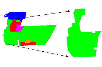
Left: Joliet Arsenal land use plan. Green areas represent Midewin. Right: Study site in the western half of Midewin.
Appendix A: Soil Series at Midewin
Appendix B: ARC/INFO GRID AML scripts for potential Prairie community restoration
Appendix C: ARC/INFO GRID AML script for restoration Prioritization
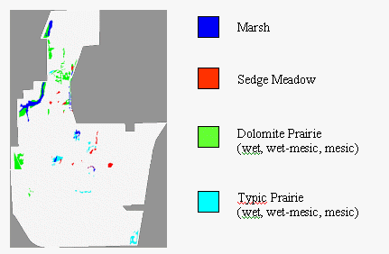
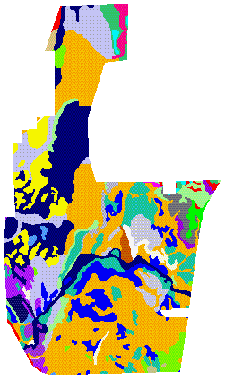
Figure 2: Existing prairie vegetation communities
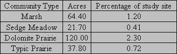
Table 1: Areas calculated for vegetation communities
Figure 3: GIS data: DOQQ and soil series
Figure 4: Creating the TCI map from the DEM
Figure 6: Classification and Regression Tree (CART)
Figure 7: Potential restoration distribution maps
Figure 8: Distance from existing vegetation
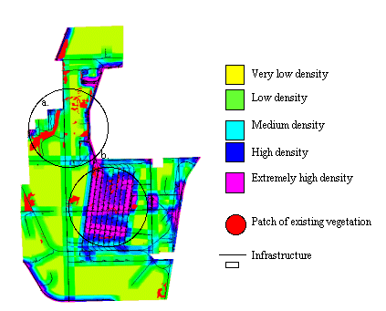
Figure 9: Infrastructure density
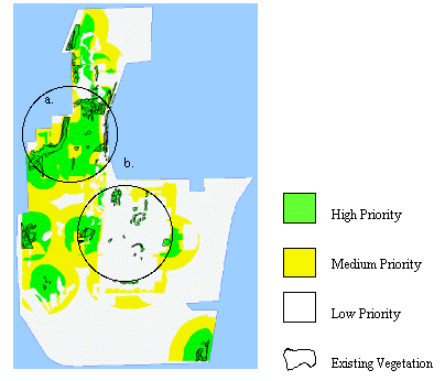
Figure 10: Restoration prioritization
Abstract
Joliet Arsenal, a decommissioned Army munitions facility in Illinois,
is being restored by the USDA Forest Service as Midewin National Tallgrass
Prairie. I used a new GIS method to help the Forest Service better utilize
complex spatial data for restoration and management. First I defined top
restoration priorities for restoration sites: existing prairie and surroundings,
good restoration potential and low infrastructure density. Then I used
ARC/INFO GRID and ran a Classification and Regression Tree analysis (CART)
to spatially quantify each priority into a coverage. Finally I combined
the coverages to create one comprehensive restoration prioritization map.
The tallgrass prairie ecosystem has a high richness and diversity of plant and animal species that, while once common, are now threatened by extreme habitat loss. Only 4% of presettlement tallgrass prairie remains in the United States (Sampson & Knopf, 1994). Since the tallgrass prairie ecosystem is maintained by natural disturbances, and these disturbances no longer occur due to the small size and isolation of remaining patches, conservation of this ecosystem requires intensive management. Furthermore, in order to conserve large patches of tallgrass prairie, ecological restoration of degraded prairie is necessary.
As larger scale projects become more widespread in ecology and conservation (Rastetter et al., 1992) Geographical Information Systems (GIS) are becoming essential tools for research and management. A successful conservation application of GIS is pairing it with Classification and Regression Tree Analysis (CART) to model vegetation and wildlife distributions based on learning samples (Walker, 1990); (Moore et al., 1991). Another emerging application in soil, water resource, and human health planning is integrating the GIS with Decision Support Systems (DSS) to form Spatial Decision Support Systems (SDSS). SDSS can help managers balance multiple management objectives in a spatially explicit manner (Montas & Madramootoo, 1992); (Lindquist et al., 1996). Similar types of decision-making are required in conservation, where SDSS has great potential.
The Conservation Fund, a nonprofit conservation organization, is developing a SDSS that aims to enhance the USDA Forest Service's restoration management of Midewin National Tallgrass Prairie in Illinois. My primary objective, as part of The Conservation Fund project, was to demonstrate potential uses of the SDSS. To accomplish this I developed a method that integrates ecological, topographic, and infrastructure data together to address salient restoration management questions, such as:
Besides internally helping the Forest Service in restoration management at Midewin, another objective for the SDSS is to encourage more interactive and consensus-building community involvement in management plans. The intention is that access to the SDSS will educate the public about Midewin which will enable them to contribute educated and constructive input to the Forest Service's restoration management plans, as well as facilitate consensus and support of the plan. The Conservation Fund has started the community involvement process by using custom GIS-derived paper maps that will eventually involve the SDSS as it is completed. The Conservation Fund has used the SDSS approach before with greenway planning in Florida (Shields & Sexton, 1996). Similarly, an ongoing project in Zambia is successfully using GIS as a tool to involve local communities in wildlife management (Lewis, 1996). Leaders have been using land use maps to educate local residents about wildlife resources and to overcome conflict and build consensus about land use decisions (ibid).
The study site is the western half of Midewin National Tallgrass Prairie, a 6329 acre (2562 hectare) piece of land in Will County, IL (see Figure 1). The elevations range from 510 to 680 feet above sea level (Glass, 1994). The topography and soils were formed in the Wisconsin glaciation, which ended around 8000 years ago, and some moraines left by the glacier are present at the site (ibid). The prairie is within the Jackson Creek, Grant Creek, Prairie Creek, Jordan Creek, Des Plaines River, and Kankakee River drainages. Jackson Creek is the largest waterway in the area, with the largest watershed and greatest water flow (ibid). According to Hite and Bertrand's 1989 biological assessment of Illinois stream quality, Jackson Creek is a highly valued aquatic resource, and one of the best in northeastern Illinois (Glass, 1994).
Left: Joliet Arsenal land use plan. Green areas represent Midewin. Right: Study site in the western half of Midewin.
Currently, there are scattered remaining patches of eight tallgrass prairie communities that have survived the land use changes at Midewin. Since prairie vegetation is extremely diverse it would be neither unrealistic nor useful to characterize each species that makes up each community type. Therefore, although species level information is critical for implementing restoration work, prairie communities are usually described by their dominant plant species. They are as follows:
Humans have modified the Midewin land in different eras. First it was used for agriculture and cattle grazing. From the 1940s to the Vietman War it was Joliet Arsenal, an Army munitions facility. The site has been mostly idle since then, and much of the land the Army (and now the Forest Service) continues to lease for agriculture (Glass 1994). Now that Midewin is part of the Forest Service, the agricultural leases are being phased out and the land will be managed first for conservation, then science and education, and lastly for recreation. At Midewin, some modern disturbances, such as railroads and roads, will be discontinued, while some historic disturbances, such as fire, and possibly Bison grazing, will be reintroduced in the hope that a tallgrass prairie, close to pre-settlement form, will once again appear.
The data I started out with were the soil map (digitized from National Soil and Conservation Service maps); unrectified aerial photos of Midewin with hand-drawn native vegetation community polygons (Ecological Services, 1995); and various state-wide data layers, such as streams, roads, and railroads, from the Illinois Division of Natural Resources. I digitized the native vegetation maps, first to mylar to get more control points and then into one large polygon coverage. The fact that the vegetation maps were unrectified, plus the extra step involving mylar, added additional error into the vegetation coverage.
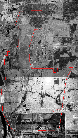
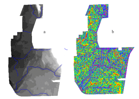
Later in the project I received rectified digital ortho photo quads (DOQQs) (Figure 3a) from the USGS along with line coverages for elevation, roads, and buildings. The new ARC coverage extents were limited to within the boundaries of Midewin National Tallgrass Prairie (the other land uses of the former Joliet Arsenal, such as the industrial parks and landfill, were not included in the coverages). Also, due to financial arrangements between the Forest Service and USGS, there was only complete data for the western half of Midewin. Therefore it happened that the western half had the best available data so I chose that half as my study area (Figure 1). Using the DOQQs (Figure 3a) I manually corrected each vegetation polygon in the study area.
3a) DOQQ's-rectified aerial photos with a resolution of 3.5 feet. 3b) Soil series map.
I projected all the coverages into the most common form: UTM, feet, Clarke 1866 and Zone 16. Once everything was in the same projection, I transformed all coverages to raster so I could use them in ARC/INFO's GRID program. Everything was transformed in 10 foot pixels, except the line elevation map, which was in 25 foot pixels because more resolution would not have affected the image, since this was less than the distance between elevation lines.
Constructing the environmental envelope
In order to determine ecological distributions for species or communities, the climatic or environmental envelope must be defined statistically, then modeled spatially. Shao and Halpin (1996) used modeling techniques to find that for eastern North American tree and shrubs, actual evapotranspiration and growing degree day indices could accurately predict species ranges. Walker (1990) used GIS and CART analysis to find the climatic envelope for three kangaroo species and found that the most important variables are precipitation and annual mean temperature. Michaelsen et al. (1994) used CART, remote sensing, and terrain data to find the environmental envelope of a tallgrass prairie in Kansas. They found that burning treatment and elevation are important variables (ibid). Likewise my aim was find the environmental envelope, from the available data, that characterizes Midewin's tallgrass prairie communities.
One variable for the environmental envelope of the Midewin plant communities is elevation. Topographic variation is an important driver in plant community ecology, even in relatively flat landscapes. Slight variations in elevation can make a critical difference in environmental conditions, which in turn influence species competition and dominance (Steinauer and Collins, 1996). Thus elevation is a critical variable in the environmental envelope.
A second variable that has a significant effect on plant community composition is surface moisture. However, it is unusual to have detailed hydrological data for a site due to the expense and time involved in collecting it. Realizing this hydrological data shortage was common, Bevin and Kirby (1979) developed TOPMODEL, a surface hydrological flow model based on topography, which is a widely available type of data. TOPMODEL finds surface water flow and drainage patterns by finding ln(a/tanB) for each point, where a is the "cumulative upslope area draining through a point," and tanB is the slope angle at that point (Beven et al, 1991). The map of ln(a/tanB) values was tested against a gauged basin with good results (Beven and Kirby, 1979) and has since been widely used in hydrologic modeling (Beven et al, 1991). Wolock (1993) developed a Topographic Convergence Index (TCI) based on TOPMODEL that converts digital elevation models into a surface drainage networks by calculating TCI = ln(a/tanB) for each cell in the grid. Calculating TCI from a digital elevation model is a way to approximate surface wetness, an important but hard to obtain environmental variable, from readily available data.
In the absence of field-derived hydrological data I used Wolock's (1993) technique in deriving a TCI map. Figure 4a is the digital elevation map from which I calculated TCI. It is apparent that the TCI map (Figure 4b) has the high wetness where the stream beds are located in the elevation map. This TCI map was used as a surface wetness map in my analysis.
4a: Digital elevation map (DEM) with streams coverage.
White is higher elevation and darker is lower.
4b: Topographic Convergence Index (TCI). Blue is wettest,
then green, yellow are drier and the driest is red.
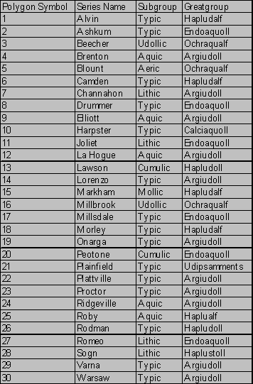
Another variable that affects plant community composition is the geology of parent materials. I used the soil map (Figure 3b) as a proxy for geology as the third and final variable in the environmental envelope. There were 30 different soil series at Midewin (Appendix A) and 17 of them, almost all Mollisols, had some of the 8 prairie types growing on them. Most of these 17 were poorly drained, and 6 were categorized as hydric.
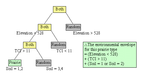
To find the environmental envelopes of the vegetation communities, using elevation, TCI and soil type as variables, I performed a Classification and Regression Tree (CART) Analysis. CART is a type statistical analysis for spatial data that develops decision rules to split data into more homogenous subsets (Walker, 1990). The first decision rule is the most statistically significant attribute value that divides the data into two groups. The second is the best split of each of those subsets. This process continues until all the data is broken up into homogenous groups. Then all the decision rules can be strung together to build a blueprint for the tree, in other words, to construct the environmental envelope. CART analysis is increasingly being utilized due to its many strengths: outliers do not distort the model, CARTs are "easy to understand and evaluate, and do not require all attributes to be present for the model to be evaluated" (ibid.) Nonetheless there are some limitations to CART analysis. Often minor changes in the learning sample can have a large effect on tree structure. Also, there is ambiguity to how many rules make up an accurate tree (ibid.)
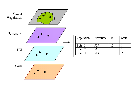
I chose CART analysis because it allowed me to model where eight prairie community types would be most successfully restored with a limited amount of environmental data. I needed a way to describe where the current prairie community types existed and to glean rules that I could use to pinpoint where else similar conditions were found, thus would have good restoration prospects. To run CART, I first sampled 10% of each vegetation type for the learning sample and generated random points for the entire study site. Then in GRID I overlaid the vegetation and random points with the three variable layers (elevation, TCI and soil). This generated a list of each point with its values for each of the three variables (Figure 5). I ran a CART for each of the eight vegetation communities. The CART output is tree with branches that split along key decision rules (Figure 6).
The trees generated from the CART analysis form the basis of the environmental envelope that can be used as a basis for constructing a habitat model for a species or plant community. I used the rules that defined the environmental envelope for each vegetation community type and found where else on the study sites these conditions occurred by turning the rules in a computer script. The script output was a GIS map of all the other cells at Midewin that matched the environmental envelope, which I call the "potential restoration map." I made a potential restoration map for each community.
CART analysis describes the environmental envelope of each prairie community type.
For the last two maps, I added the potential restoration maps from all three vegetation communities into one that shows where there is one, two or three communities predicted for each cell. Overall, dolomite is predicted on lower elevation than typic, and is associated with different soil types.
7 (a, b) Green is predicted vegetation. 7a. Potential
marsh. 7b. Potential sedge meadow.
7 (c, d) Red is one type, yellow is two and green is
three types. 7c. Dolomite prairie. 7d. Typic prairie.
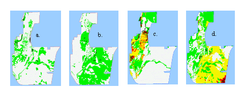
When using only three variables in an environmental envelope only a rough approximation can be drawn. As is apparent in Figure 7 the potential restoration maps overlap one another. Some vegetation types, such as mesic typic prairie, had too few sample points, which resulted in an oversimplified tree (Appendix B). This made the environmental envelope too general, and will likely make its prediction power weak. This may be alleviated by adding more sample points, or by using additional variables in the environmental envelope. Other vegetation types, such as marsh, were well represented and had a tighter envelope (Figure 7a, Appendix B), which will likely result in better prediction power. In future work, one way to try to decrease the overlap would be to do a CART analysis among different types of prairie vegetation points instead of between prairie vegetation points and a random points (the way I did it.) This would force the CART to choose splitting rules between vegetation types. Instead of a separate potential restoration map for each vegetation type, the result would be a single map with each vegetation type demarcated. There may be a limit to how well this would work because prairie community boundaries are not sharp, but are continuous ecotones, so some overlap between types is unavoidable. In addition, if these are truly areas that can support many communities, they may be ideal areas to grow prairie seed. Nonetheless, all of the envelopes will likely become finer as additional data becomes available, such as fire and grazing treatment, and as the data is corroborated with field measurements.
To demonstrate how a Spatial Decision Support System (SDSS) can be used to make decisions based on explicitly stated priorities, I constructed a sample restoration prioritization map as input to the SDSS. This map is based on priorities that I assumed, for demonstration purposes, would be similar to actual Forest Service priorities. As additional data becomes available priority layers can be weighted to reflect current conditions and be added to or deleted from the SDSS.
My sample prioritization map combines the following assumed priorities: 1) conserving existing native prairie vegetation, 2) conserving areas surrounding existing vegetation, 3) restoring sites with low infrastructure density and 4) restoring sites with good restoration potential. In order to turn these priorities into a single map, each priority had to first be mapped separately. Existing native prairie communities, important to conserve, already existed in the form of the native vegetation map. Areas surrounding the existing vegetation, which would maximize natural dispersal, needed to be represented spatially. Potential restoration distributions were already mapped from the CART analysis. I combined the eight potential restoration maps into a single potential restoration map for all prairie vegetation. Finally, sites with the least existing infrastructure, areas where restoration efforts have the least physical obstacles, needed to be mapped as well.
Yellow is the closest and red is the farthest. Existing
native vegetation patches are outlined in black.
8a & b have a high concentration of sites close to
existing vegetation.
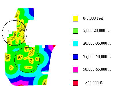
In GRID I constructed a continuous surface distance map from all the native vegetation patches (Figure 8). Distance surfaces can be used to model natural seed dispersal, which is important to consider when undertaking a large restoration project. Values calculated from maximum dispersal distance can be used as thresholds in a prioritization model.
Restoration is an applied science. One must take into account many factors besides strictly ecological ones that make a site better or worse for restoration. For example, if an area has wide open spaces it may be better for prescribed burning than one with buildings and railroad tracks. It would be expensive and take longer to get rid of these structures before restoring vegetation. However, the same characteristics that make poor restoration sites can be assets for recreation areas. Using the same example, railroad beds can be turned into hiking trails and buildings into shelters for recreation. This would save resources by not having to tear the infrastructure down or build from scratch. Using this line of reasoning I created an infrastructure density map. To make the map I added roads and buildings together in GRID then passed a moving window over each cell the combined grid. The window took the mean infrastructure value of that square of cells and assigned it to middle cell. The resulting GRID is an infrastructure density map (Figure 9).
Yellow and green are the lowest infrastructure densities
and purple and blue are the highest densities.
9a has a low density and 9b has a high density.
I combined the four management priority maps; existing native vegetation, distance from existing vegetation, potential restoration, and infrastructure density, into an aggregated restoration priority map (Figure 10 & Appendix C). I created the final restoration priority map using the following rules:
Compare Circles a and b from Figures 8-10. Circle a has lots of existing native vegetation in close proximity and has low infrastructure density, which put it in the highest priority class for restoration. In contrast, Circle b also has existing vegetation in close proximity, but has extremely high infrastructure density, thus it was put into the lowest priority class. Restoration has to start somewhere. This restoration priority map can help managers decide where to begin restoration efforts. High priority areas are good places to do field assessments for restoration potential. Low priority areas can be seen as long range restoration goals or as options for recreation areas.
Green areas are high priority because they have or are close to existing vegetation, has restoration potential, and have little infrastructure. White areas are low priority because they have no existing vegetation, are far from existing vegetation, have little restoration potential, and/or have high infrastructure. Yellow areas are intermediate between the high and low. 10a) High priority area. 10b) Low priority area except for patches of existing vegetation.
The method I have applied in this project to create the restoration prioritization map combines relevant information to help guide decision-making. The intention is that these methods and maps will be integrated into TCF's SDSS to be used at Midewin. As part of an SDSS, priorities can be weighed in different ways from what I have demonstrated in this project. SDSS' can aid restoration management decisions by spatially depicting multiple priorities. In addition, since prioritization assumptions are explicit and the final product is easily understood, SDSS' can be used to encourage public participation and consensus on management plans. I demonstrated a method that could be useful to the Forest Service in both restoration management and community involvement. However, to be accurate enough to be useful at site level scale, the data that goes into each layer of the GIS must be more detailed and tested in the field. A GIS model cannot be any more accurate that the data that goes into it. However, despite these caveats, my prioritization method as part of an SDSS has enormous potential for restoration management.
Allen, T.F.H. and E.P. Wyleto. 1983. A hierarchical model for the complexity of plant communities. Journal of Theoretical Biology 101:529-540.
Allen, W. 1997. Personal communication.
Bevin and Kirby. 1979. A physically based, variable contributing area model of basin hydrology. Hydrological Sciences Bulletin 24(1):43-69.
Collins, S.L. Interactions of disturbances in tallgrass prairie: A field experiment. Ecology 68(5):1243-1250.
Crupi, C. 1995-7. Personal communications and internal memos.
Diamond, H.L. and P.F. Noonan. 1996. Land Use in America. Washington DC: Island Press. 351p.
Ecological Services. 1995. Native Vegetation at the Joliet Army Ammunition Plant and Joliet Training Area. Prepared for the Illinois Department of Conservation (unpublished.)
Glass, W.D. 1994. A Survey of the Endangered and Threatened Plant and Animal Species of the Joliet Army Ammunition Plant and Joliet Training Area-Will County, IL. Division of Natural Heritage, Illinois Department of Conservation. Springfield, IL (unpublished.)
Herkert, J.R. 1994. The effects of habitat fragmentation on Midwestern grassland bird communities. Ecological Applications 4(3):461-471.
Hite, R.L. and B.A. Bertrand. 1989. Biological stream characterization (BSC): A biological assessment of Illinois stream quality. Illinois State Water Plan Task Force Special Report 13:1-42.
Howe, H.F. 1994a. Response of early- and late-flowering plants to fires season in experimental prairies. Ecological Applications 4(1):121-133.
Howe, H.F. 1994b. Managing Species Diversity in Tallgrass Prairie: Assumptions and Implications. Conservation Biology 8(3):691-704.
Howe, H.F. 1995. Succession and Fire Season in Experimental Prairie Plantings. Ecology 76(6):1917-1925.
Jenson, S.K. 1991. Applications of hydrological information automatically extracted from digital elevation models. Hydrological Processes. 5:31-44.
Kelting, R.W. 1954. Effects of moderate grazing on the composition and plant production of a native tall-grass prairie in central Oklahoma. Ecology 35:200-207.
Knopf, F.L. 1996. Prairie Legacies-Birds. Prairie Conservation: Preserving North America's Most Endangered Ecosystem. Washington, DC: Island Press. pp135-148
Lewis, D.M. 1996. Importance of GIS to community-based management of wildlife: Lessons from Zambia. Ecological Applications 5(4): 861-871.
Lindquist, K., M. McGee, and L. Cole. 1996. TVA-EPRI River Resource Aid (TERRA) reservoir and power operations decision support system. Water Air and Soil Pollution 90(1-2): 143-150.
Michaelson, J., D.S. Schimel, M.A. Friedl, F.W. Davis, and R.C. Dubayah. 1994. Regression Tree Analysis of satellite and terrain data to guide vegetation sampling and surveys. Journal of Vegetation Science 5:673-686.
Montas, H. and C.A. Madramootoo. 1992. A decision support system for soil conservation planning. Computers and Electronics in Agriculture 7(3): 187-202.
Moore, D.M., B.G. Lees, and S.M. Davey. 1991. A New Method for Predicting Vegetation Distributions using Decision Tree Analysis in a Geographical Information System. Environmental Management 15: 59-71.
National Wildlife Service. 1993. Memo.
O'Keefe, Joyce. August 1997. Personal communication.
Ratstetter, E.B., A.W. King, B.J. Cosby, G.M. Hornberger, R.V. O'Neill, and J.E. Hobbie. 1992. Ecological Applications 2(1): 55-70.
Samson, F.B., and F.L. Knopf. 1994. Prairie conservation in North America. BioScience 44(6):418-421.
Samson, F.B., and F.L. Knopf. 1996. Prairie Conservation: Preserving North America's Most Endangered Ecosystem. Washington, DC: Island Press.
Shao, G. and P.N. Halpin. 1996. Climatic controls of eastern North American coastal tree and shrub distributions. Journal of Biogeography 22:1083-1089.
Shields, E. and M. Sexton. 1996. Loxahatchee Greenways Project. Land Use in America. Washington DC: Island Press. pp.129-131.
Steuter, A.A.. 1991. Human impacts on biodiversity in America: Thoughts from the Grassland Biome." Conservation Biology 5:136-37.
Steinauer, E.M. and S.L. Collins. 1996. Prairie Ecology-The Tallgrass Prairie. Prairie Conservation: Preserving North America's Most Endangered Ecosystem. Washington, DC: Island Press. pp.39-52
The Conservation Fund. 1994. MacArthur Grant Application. (unpublished)
Walker, P.A. 1990. Modelling wildlife distributions using a geographical information system: kangaroos in relation to climate. Journal of Biogeography 17:279-289.
Wolock, D. 1993. Simulating the variable-source-area concept of streamflow generation with the watershed model TOPMODEL. USGS Water-Resources Investigation Report. 93-XXXX.
Pat Halpin, Advisor
The Conservation Fund
Gwynn Crichton
APPENDIX A: SOIL SERIES AT MIDEWIN
Appendix B: ARC/INFO GRID AML scripts for potential Prairie community restoration
Derived from S PLUS Classification and Regression Trees (CART)
Potential marsh (Typha latifolia and Scirpus atrovirens):
docell
if (elev < 527.98 & tci < 105.5 & elev > 525.405)
veg1_predict = 1
else if (elev < 527.98 & tci > 105.5)
veg1_predict = 1
else if (elev > 527.98 & (soil == 8 or soil == 11 or soil == 23 or soil == 24 or soil == 27) & soil == 8 & elev > 537.995 & elev < 540.546 & elev < 540.013 & tci > 84.5)
veg1_predict = 1
else if (elev > 527.98 & (soil == 8 or soil == 11 or soil == 23 or soil == 24 or soil == 27) & soil == 8 & elev > 537.995 & elev < 540.546 & elev > 540.013)
veg1_predict = 1
else if (elev > 527.98 & (soil == 8 or soil == 11 or soil == 23 or soil == 24 or soil == 27) & (soil == 11 or soil == 23 or soil == 24 or soil == 27) & elev < 533.077)
veg1_predict = 1
else if (elev > 527.98 & (soil == 8 or soil == 11 or soil == 23 or soil == 24 or soil == 27) & (soil == 11 or soil == 23 or soil == 24 or soil == 27) & elev > 533.077 & elev > 541.839)
veg1_predict = 1
else if (elev > 527.98 & (soil == 8 or soil == 11 or soil == 23 or soil == 24 or soil == 27) & (soil == 11 or soil == 23 or soil == 24 or soil == 27) & elev > 533.077 & elev < 541.839 & elev < 537.178 & tci < 94.5 & elev > 534.013 & tci > 73 & elev < 534.478)
veg1_predict = 1
else if (elev > 527.98 & (soil == 8 or soil == 11 or soil == 23 or soil == 24 or soil == 27) & (soil == 11 or soil == 23 or soil == 24 or soil == 27) & elev > 533.077 & elev < 541.839 & elev < 537.178 & tci < 94.5 & elev > 534.013 & tci < 73)
veg1_predict = 1
else if (elev > 527.98 & (soil == 8 or soil == 11 or soil == 23 or soil == 24 or soil == 27) & (soil == 11 or soil == 23 or soil == 24 or soil == 27) & elev > 533.077 & elev < 541.839 & elev < 537.178 & tci < 94.5 & elev < 534.013 & tci > 75.5 & elev < 533.993 & elev > 533.306)
veg1_predict = 1
else veg1_predict = 0
end
Potential sedge meadow (Carex stricta and Eupatorium maculatum):
docell
if ((soil == 1 or soil == 8 or soil == 11 or soil == 16 or soil == 19 or soil == 23 or soil == 26) & elev < 543.176 & soil == 8 & elev > 534.68 & tci > 83.5 & elev < 540.875 & elev < 537.546 & elev < 535.865)
veg2_predict = 1
else if ((soil == 1 or soil == 8 or soil == 11 or soil == 16 or soil == 19 or soil == 23 or soil == 26) & elev < 543.176 & soil == 8 & elev > 534.68 & tci > 83.5 & elev < 540.875 & elev > 537.546 & tci > 94)
veg2_predict = 1
else if ((soil == 1 or soil == 8 or soil == 11 or soil == 16 or soil == 19 or soil == 23 or soil == 26) & elev < 543.176 & soil == 8 & elev > 534.68 & tci > 83.5 & elev > 540.875)
veg2_predict = 1
else if ((soil == 1 or soil == 8 or soil == 11 or soil == 16 or soil == 19 or soil == 23 or soil == 26) & elev < 543.176 & (soil == 11 or soil == 26) & elev > 533.3)
veg2_predict = 1
else if ((soil == 1 or soil == 8 or soil == 11 or soil == 16 or soil == 19 or soil == 23 or soil == 26) & elev > 543.176)
veg2_predict = 1
else veg2_predict = 0
end
Potential dolomite prairie:
docell
if (elev < 538.982 & elev < 528.503 & elev > 523.988 & tci < 66 & elev < 526)
veg4_predict = 1
else if (elev < 538.982 & elev < 528.503 & elev > 523.988 & tci > 66)
veg4_predict = 1
else if (elev < 538.982 & elev > 528.503 & (soil == 10 or soil == 11 or soil == 19 or soil == 26 or soil == 27))
veg4_predict = 1
else if (elev < 538.982 & elev > 528.503 & (soil == 7 or soil == 8 or soil == 17 or soil == 30) & elev < 536.833 & elev < 531.416 & (soil == 8 or soil == 17) & tci > 77.5 & soil == 17)
veg4_predict = 1
else if (elev < 538.982 & elev > 528.503 & (soil == 7 or soil == 8 or soil == 17 or soil == 30) & elev > 536.833 & soil == 8)
veg4_predict = 1
else veg4_predict = 0
end
Potential typic prairie:
docell
if ((soil == 4 or soil == 8 or soil == 10 or soil == 11 or soil == 20 or soil == 23 or soil == 26) & elev < 549.979 & (soil == 4 or soil == 20 or soil == 23))
veg5_predict = 1
else if ((soil == 4 or soil == 8 or soil == 10 or soil == 11 or soil == 20 or soil == 23 or soil == 26) & elev < 549.979 & (soil == 8 or soil == 10 or soil == 11 or soil == 26) & elev < 533.734 & elev < 531.228 & tci < 92.5)
veg5_predict = 1
else if ((soil == 4 or soil == 8 or soil == 10 or soil == 11 or soil == 20 or soil == 23 or soil == 26) & elev < 549.979 & (soil == 8 or soil == 10 or soil == 11 or soil == 26) & elev > 533.734 & elev < 534.878)
veg5_predict = 1
else if ((soil == 4 or soil == 8 or soil == 10 or soil == 11 or soil == 20 or soil == 23 or soil == 26) & elev < 549.979 & (soil == 8 or soil == 10 or soil == 11 or soil == 26) & elev > 533.734 & elev > 534.878 & elev > 537.64 & tci > 85.5)
veg5_predict = 1
else if ((soil == 4 or soil == 8 or soil == 10 or soil == 11 or soil == 20 or soil == 23 or soil == 26) & elev > 549.979)
veg5_predict = 1
else veg5_predict = 0
end
Potential wet dolomite prairie (Deschampsia caespitosa and Calamagrostis canadensis):
docell
if (elev < 527.981)
veg6_predict = 1
else if (elev > 527.981 & (soil == 5 or soil == 7 or soil == 8 or soil == 13 or soil == 17 or soil == 18 or soil == 26) & elev < 538.61 & elev > 537.114 & soil == 8)
veg6_predict = 1
else if (elev > 527.981 & (soil == 10 or soil == 11 or soil == 12 or soil == 19 or soil == 27) & elev < 537.365 & elev > 532.917)
veg6_predict = 1
else veg6_predict = 0
end
Potential wet-mesic dolomite prairie (Panicum virgatum and Solidago riddellii):
docell
if (elev < 528.495)
veg7_predict = 1
else if (elev > 528.495 & elev < 539.629 & (soil == 7 or soil == 8 or soil == 10 or soil == 17) & (soil == 8 & soil == 10) & elev < 537.351 & elev < 534.508 & elev > 530.073 & elev < 531.868)
veg7_predict = 1
else if (elev > 528.495 & elev < 539.629 & (soil == 7 or soil == 8 or soil == 10 or soil == 17) & (soil == 8 & soil == 10) & elev < 537.351 & elev < 534.508 & elev > 530.073 & elev > 531.868 & elev > 533.502 & elev < 533.839)
veg7_predict = 1
else if (elev > 528.495 & elev < 539.629 & (soil == 7 or soil == 8 or soil == 10 or soil == 17) & (soil == 8 & soil == 10) & elev < 537.351 & elev < 534.508 & elev > 530.073 & elev > 531.868 & elev > 533.502 & elev > 533.839 & tci > 91 & tci < 105)
veg7_predict = 1
else if (elev > 528.495 & elev < 539.629 & (soil == 7 or soil == 8 or soil == 10 or soil == 17) & (soil == 8 & soil == 10) & elev > 537.351 & elev < 537.585)
veg7_predict = 1
else if (elev > 528.495 & elev < 539.629 & (soil == 7 or soil == 8 or soil == 10 or soil == 17) & (soil == 8 & soil == 10) & elev > 537.351 & elev > 537.585 & elev > 538.077 & elev < 539.1)
veg7_predict = 1
else if (elev > 528.495 & elev < 539.629 & (soil == 7 or soil == 8 or soil == 10 or soil == 17) & (soil == 7 & soil == 17) & elev < 530.802 & soil == 17 & tci > 78.5)
veg7_predict = 1
else if (elev > 528.495 & elev < 539.629 & (soil == 11 or soil == 19 or soil == 26 or soil == 27) & elev > 530.84 & elev < 536.318 & (soil == 11 or soil == 26) & elev < 533.994 & elev < 533.943 & tci < 82.5)
veg7_predict = 1
else if (elev > 528.495 & elev < 539.629 & (soil == 11 or soil == 19 or soil == 26 or soil == 27) & elev > 530.84 & elev < 536.318 & (soil == 11 or soil == 26) & elev < 533.994 & elev < 533.943 & tci > 82.5 & elev < 533.531 & elev < 533.35 & tci > 109.5)
veg7_predict = 1
else if (elev > 528.495 & elev < 539.629 & (soil == 11 or soil == 19 or soil == 26 or soil == 27) & elev > 530.84 & elev < 536.318 & (soil == 11 or soil == 26) & elev < 533.994 & elev < 533.943 & tci > 82.5 & elev > 533.531 & elev < 533.9 & tci < 99)
veg7_predict = 1
else if (elev > 528.495 & elev < 539.629 & (soil == 11 or soil == 19 or soil == 26 or soil == 27) & elev > 530.84 & elev < 536.318 & (soil == 11 or soil == 26) & elev < 533.994 & elev > 533.943)
veg7_predict = 1
else if (elev > 528.495 & elev < 539.629 & (soil == 11 or soil == 19 or soil == 26 or soil == 27) & elev > 530.84 & elev < 536.318 & (soil == 11 or soil == 26) & elev > 533.994 & elev > 534.211 & elev < 534.369)
veg7_predict = 1
else if (elev > 528.495 & elev < 539.629 & (soil == 11 or soil == 19 or soil == 26 or soil == 27) & elev > 530.84 & elev < 536.318 & (soil == 11 or soil == 26) & elev > 533.994 & elev > 534.211 & elev > 534.369 & elev < 535.999 & elev > 535.932 & tci < 95.5 & tci < 88.5 & elev > 534.564 & elev < 535.454)
veg7_predict = 1
else if (elev > 528.495 & elev < 539.629 & (soil == 11 or soil == 19 or soil == 26 or soil == 27) & elev > 530.84 & elev < 536.318 & (soil == 11 or soil == 26) & elev > 533.994 & elev > 534.211 & elev > 534.369 & elev < 535.999 & elev > 535.932 & tci > 95.5 & elev < 535.501)
veg7_predict = 1
else if (elev > 528.495 & elev < 539.629 & (soil == 11 or soil == 19 or soil == 26 or soil == 27) & elev > 530.84 & elev < 536.318 & (soil == 11 or soil == 26) & elev > 533.994 & elev > 534.211 & elev > 534.369 & elev > 535.999 & elev < 536.096)
veg7_predict = 1
else if (elev > 528.495 & elev < 539.629 & (soil == 11 or soil == 19 or soil == 26 or soil == 27) & elev > 530.84 & elev < 536.318 & (soil == 19 or soil == 27))
veg7_predict = 1
else if (elev > 528.495 & elev < 539.629 & (soil == 11 or soil == 19 or soil == 26 or soil == 27) & elev > 530.84 & elev > 536.318 & tci > 72.5 & elev < 537.749)
veg7_predict = 1
else veg7_predict = 0
end
Potential mesic dolomite prairie (Andropogon gerandii and Eryngium yuccifolium):
docell
if ((soil == 11 or soil == 13 or soil == 17 or soil == 18) & elev > 530.791)
veg8_predict = 1
else if (soil == 7 or soil == 27)
veg8_predict = 1
else veg8_predict = 0
end
Potential wet typic prairie (Spartina pectinata and Lycopus americanus):
docell
if ((soil == 4 or soil == 8 or soil == 10 or soil == 11 or soil == 20 or soil == 23 or soil == 26) & elev < 540.44 & (soil == 8 or soil == 10 or soil == 11) & elev < 534.443 & elev < 533.939 & elev < 531.006)
veg9_predict = 1
else if ((soil == 4 or soil == 8 or soil == 10 or soil == 11 or soil == 20 or soil == 23 or soil == 26) & elev < 540.44 & (soil == 8 or soil == 10 or soil == 11) & elev < 534.443 & elev > 533.939)
veg9_predict = 1
else if ((soil == 4 or soil == 8 or soil == 10 or soil == 11 or soil == 20 or soil == 23 or soil == 26) & elev < 540.44 & (soil == 23 or soil == 26))
veg9_predict = 1
else if ((soil == 4 or soil == 8 or soil == 10 or soil == 11 or soil == 20 or soil == 23 or soil == 26) & elev > 540.44)
veg9_predict = 1
else if (soil == 5 or soil == 13 or soil == 17 or soil == 18 or soil == 27)
veg9_predict = 1
else veg9_predict = 0
end
Potential wet-mesic typic prairie (Panicum virgatum and Eupatorium perfoliatum):
docell
if ((soil == 8 or soil == 10 or soil == 11 or soil == 23 or soil == 26) & elev < 537.897 & (soil == 10 or soil == 11) & elev > 533.716 & elev < 534.001)
veg10_predict = 1
else if ((soil == 8 or soil == 10 or soil == 11 or soil == 23 or soil == 26) & elev < 537.897 & (soil == 8 or soil == 26) & elev < 535.975 & elev > 532.694 & elev > 533.962 & tci < 90.5 & elev < 534.538 & elev > 534.238)
veg10_predict = 1
else if ((soil == 8 or soil == 10 or soil == 11 or soil == 23 or soil == 26) & elev < 537.897 & (soil == 8 or soil == 26) & elev < 535.975 & elev > 532.694 & elev > 533.962 & tci < 90.5 & elev > 534.538)
veg10_predict = 1
else if ((soil == 8 or soil == 10 or soil == 11 or soil == 23 or soil == 26) & elev < 537.897 & (soil == 8 or soil == 26) & elev < 535.975 & elev > 532.694 & elev > 533.962 & tci > 90.5)
veg10_predict = 1
else if ((soil == 8 or soil == 10 or soil == 11 or soil == 23 or soil == 26) & elev < 537.897 & (soil == 8 or soil == 26) & elev > 535.975 & elev > 537.488)
veg10_predict = 1
else if ((soil == 8 or soil == 10 or soil == 11 or soil == 23 or soil == 26) & elev > 537.897)
veg10_predict = 1
else veg10_predict = 0
end
Potential mesic typic prairie (Sporobolus heterolepis and Silphium terebinthinaceum):
docell
if (soil == 10)
veg11_predict = 1
else veg11_predict = 0
end
Appendix C: ARC/INFO GRID AML script for restoration Prioritization
if ((veg_study3 == 1 or veg_study3 == 2 or veg_study3 == 4 or veg_study3 == 5) or (veg1-11_dist < 1000 & predicted4 == 1 & infra_den2 < .025))
veg_test2 = 1
else if (veg1-11_dist < 2000 & predicted4 == 1 & infra_den2 < .05)
veg_test2 = 2
else veg_test2 = 3
end
Laura J. Pinnas
Master of Environmental Management
GIS; Remote Sensing; Conservation Science and Planning