Jill A. Heller, D. Phillip Guertin, Scott N. Miller, and Jeffry J. Stone

ABSTRACT

INTRODUCTION

Issues of water supply and water quality are major concerns for all people, particularly denizens of arid and semi-arid regions, and water is a limiting factor for sustaining life in the Southwestern United States. The town of Arivaca, Arizona has significant water supply problems. Recently, land owners in the Arivaca Valley have expressed concern that the water supply will be adversely impacted as new water right claims are filed or existing water rights are fully exercised.

Issues relating to water supply in Arivaca are not new. In the 1970s, consulting hydrologists assessed the characteristics of the Arivaca Creek Watershed and compiled "The Arivaca Area Plan." The purpose of the study was to determine the potential volume of water which could safely be developed for use without disrupting the ecologic balance of the watershed (Manera, 1973). The investigation concluded that a given amount of development could take place with little to no harmful effect on the basin. Since then, development has occurred and concerns once again surfaced as to the status of the water supply in the basin, in particular the portion available for recharge to the aquifer.

Groundwater recharge to the Arivaca aquifer is driven by summer monsoonal rains and winter frontal storms. Losses due to evaporation and transpiration are high. Osterkamp et al. (1994), using a study area similar to Arivaca, found recharge to be greatest in the upper portions of the watersheds where precipitation and runoff potential are the greatest. Recharge is consequently lower in lower watershed areas with less rainfall.

Osterkamp et al. (1994) estimated that, given 180 mm of annual precipitation, 1.6% recharges the groundwater reservoir, and 90% of the estimated recharge occurs by transmission loss in stream channels. The remaining 10% is accounted for as infiltration though the root zone in the upland and interchannel areas. Renard (1970) stated that for an annual precipitation amount of 305mm at Walnut Gulch, Arizona, approximately 44mm are transmission losses, of which 22mm reach the groundwater table, with the rest returning to the atmosphere through evapotranspiration.

Stockponds have been found to have a significant effect on the volume of runoff and, through decreased transmission losses, recharge, on a watershed (Sauer and Masch, 1969; Lovely, 1976; Almestad, 1983). Potential groundwater recharge into an aquifer is considered to occur primarily in ephemeral alluvial stream channels (Osterkamp et al., 1994). Therefore, reducing the amount of water that enters a downstream alluvial channel implies a loss of potential groundwater recharge.

Geographic Information Systems (GIS’s) are being widely used in hydrology and are well suited to developing input to distributed-runoff simulation models because of the inherent spatial distribution of physical characteristics such as soils, vegetation, elevation and slope. In this study, GIS played a key role in documenting the hydrologic characteristics of the Arivaca watershed and providing input to a complex distributed model, which can now be used as a basis for continued research in the area.

The motivation for this research was to gain an understanding of the hydrology of the watershed in order to provide information that will facilitate scientifically-based decision-making in the future. Our objectives were to characterize the physical, biological, hydrological, and cultural components of the watershed, synthesize the data using a surface water model, and evaluate the potential implications of stock ponds on the potential recharge in the watershed.

Historical precipitation records were assembled along with pertinent GIS theme layers to fully characterize the hydrology of the watershed. Hydrologic parameter input values were derived from the GIS theme layers. The hydrologic model, ARiD BaSiN (ARDBSN; Stone et al., 1986), coupled with a stochastic weather generator (CLIGEN; Nicks et al., 1995), was applied to simulate the hydrology of the Arivaca Creek Watershed. The effect of surface storage by stock ponds on downstream recharge potential was estimated through an analysis of runoff and transmission losses. While these results are preliminary, this study will be expanded and eventually incorporated into a decision support tool for future water and land use practices.

STUDY SITE DESCRIPTION

Arivaca Creek Watershed is located in southeastern Arizona, approximately 85 kilometers southwest of Tucson (Figure 1). 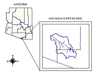The total drainage area of the watershed is approximately 120 km², which ranges in elevation from 1050m to 1350m. The climate is semi-arid with a mean annual precipitation of 394 mm. Rainfall occurs predominantly at two distinct times of year, winter and summer. Snowfall is not a significant factor. The main stream of the watershed, Arivaca Creek, is approximately 25 km in length with some perennial reaches and has six major ephemeral tributaries. Based on the Arizona Gap Analysis vegetation data (NBS – Cooperative Park Studies Unit), the vegetation of Arivaca is mainly semidesert mixed grass-mesquite with some encinal mixed oak-mesquite at the higher elevations (classified as Semidesert Grassland and Madrean Evergreen Woodland, respectively by Brown and Lowe, 1980). Arivaca is part of the Basin and Range physiographic province, characterized by steeply rising mountain ranges surrounding alluvium filled valleys (Fenneman, 1931).

MODEL DESCRIPTION

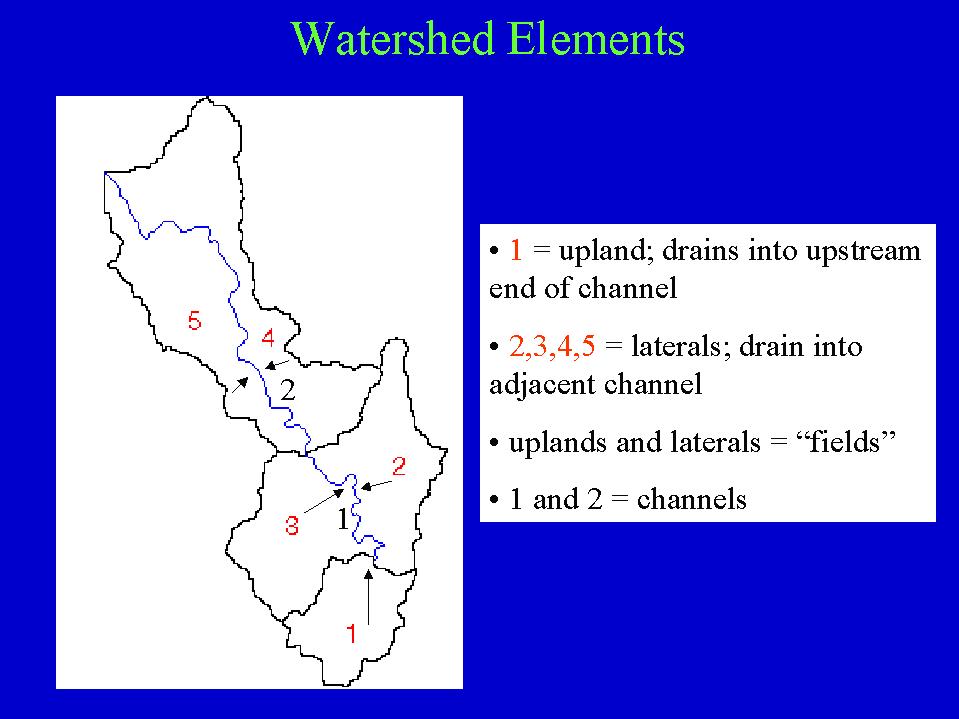
The ARDBSN model is a physically-based distributed hydrologic simulation model. Hydrologic response is computed on a daily time step, and ARDBSN is designed to run continuously over a long period of record (up to several decades) in order to be suitable as a strategic planning tool. The model is capable of predicting runoff volume and peak, as well as erosion and sediment yield. For modeling purposes, a watershed is subdivided into a series of upland, lateral, and channel elements Figure 2. The hydrology component is computed using a modified Curve Number method that incorporates the elements’ hydrologic characteristics. Runoff is routed through the various elements accounting for any pond detention, and channel runoff and volume estimates are adjusted for transmission losses.

Reasons for selecting the ARDBSN model for this study were that it runs on a daily timestep, is applicable to ungaged areas, and is designed for small semiarid rangeland watersheds. In addition, the runoff output values were viewed as a preliminary source to make relative comparisons of potential groundwater recharge to the system both with and without the factor of stock tanks.

MODEL PARAMETERIZATION

The required input for the ARDBSN model includes daily precipitation generated by the CLIGEN weather simulator, general topographic characteristics based on a Digital Elevation Model (DEM), including subcatchment properties and routing sequence, soil properties based on State Soils Geographic (STATSGO) database, vegetation data based on the Arizona Gap Analysis Vegetation Map, and a stockpond map (Figure 3).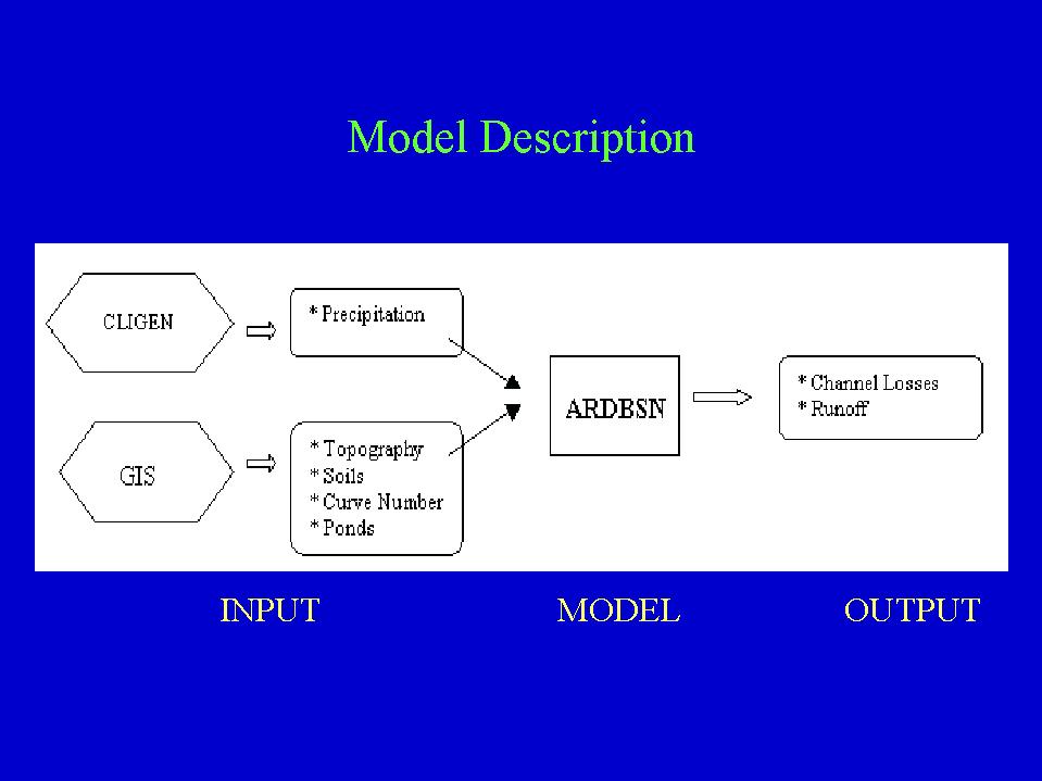

Precipitation is the most sensitive input parameter to the ARDBSN model. Therefore, it was imperative that the precipitation input be robust to assure the greatest possible confidence in the model output. A database was used to compile historical daily precipitation data for Arivaca and a thorough statistical analysis was performed on the data. The statistical analysis ensures that the generated precipitation data are representative of the actual data. An input file to the CLIGEN stochastic weather generator model was developed based on precipitation data from the Arivaca area. The simulated precipitation statistics compare quite well with historical data in terms of average annual precipitation, average monthly precipitation amount, event size distribution, and average number of annual events (Figure 4)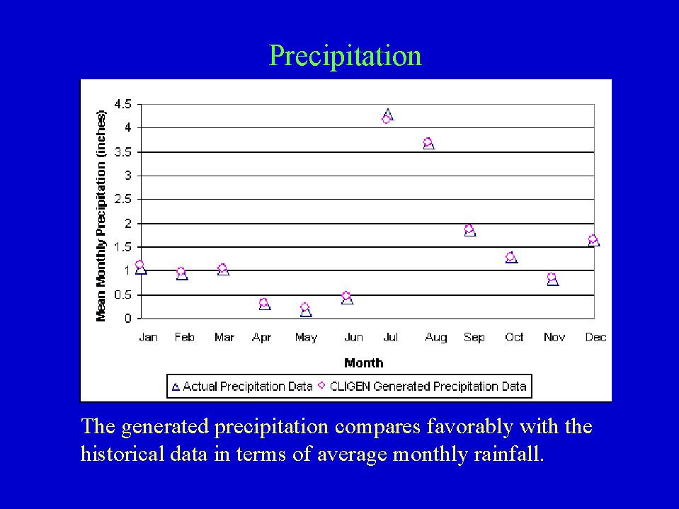. A precipitation event is considered to be at least 0.01 inches (0.254mm).

CLIGEN assumes a left-skewed normal distribution (Nicks et al., 1995). (Figure 5)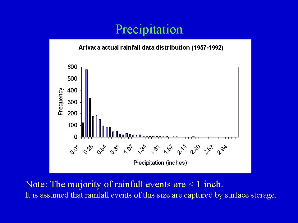 illustrates that the actual data have the assumed distribution. Osborn et al. (1972) determined optimum rain gage spacing to accurately estimate the spatial variability of rainfall in southeastern Arizona to be 2.5 km (1.5 miles). Therefore, the random seed function of CLIGEN was utilized in order to generate independent precipitation data for each of the sub-basin fields that are of proper size. Each field requires daily rainfall data for the ARDBSN input file.

A Digital Elevation Model (DEM) was the source from which the subwatershed and channel configurations were derived. Minimal smoothing was applied to the DEM data, from which flow direction and accumulation maps were derived using standard GIS techniques (Esri, 1999). An Arc Macro Language (AML) program was built which automates the creation of subcatchments within a given watershed, in a form required by ARDBSN. A copy of this AML (subws.aml) can be found in Appendix I.

Routing sequences and geometric characteristics were extracted from the subdivided watershed elements (Figure 2) and input to the ARDBSN model. The average slope for each channel in the subwatershed was calculated as the elevation difference between segment ends divided by the total stream segment length. An AML was created which used the DEM as well as the subwatershed polygon map to calculate the modified USLE length-slope (LS) factor for each field in the subwatershed. A copy of this AML (ls.aml) can be found in Appendix II.

As previously stated, the watershed is subdivided into a series of upland, lateral, and channel elements (also referred to as "fields"). For modeling purposes, each field must be linked to a channel (Wight and Skiles, 1987). An upland field drains into the upstream end of a channel while a lateral field drains into an adjacent channel.

Soil properties for each field were derived from the STATSGO soils map. An AML which uses a look-up table concept to convert the STATSGO ‘layer’ info file to a number of hydrologic modeling parameters was employed (texture1.aml; Appendix III). The soil property values used in this AML to generate parameter values are based on Wight and Skiles (1987). To prepare the STATSGO data for this AML, necessary attributes were added based on soil texture, including bare soil evaporation, porosity, 1/3 and 15 bar soil moisture retention, and saturated hydraulic conductivity (K_sat).

In STATSGO, each map unit (MUID) can have multiple components and each component can have multiple layers. The decision was made to only use the dominant texture for each soil layer for each soil type within an MUID. The decision was also made to consistently divide the soil layers into the same depths for all areas. Therefore, the values associated with the dominant texture within each soil layer (0-3", 3-6", 6-15", 15-24", 24-33", 33-42", 42-51", 51-60"; where " = inches) were assigned to that layer. Thus, soil properties were weighted by horizon and depth.

To obtain the percentage of each soil association in each field, the soils and the fields coverages were intersected, and the resultant coverage geometric data were output to a spreadsheet. The area of each MUID in a certain field was divided by the total area of the field, resulting in the percent of that MUID in that field element. This percentage was then multiplied by the soil property values previously calculated for the respective soil associations (MUIDs) and the values summed to obtain one weighted value for each soil parameter in each field for each of the eight soil layers. The soil parameters calculated in this way were porosity, 1/3 and 15 bar soil moisture retention, and K_sat. These values were input to the ARDBSN parameter input file. The bare soil evaporation factor was calculated in a similar fashion, however the this parameter only applies to the surface texture and therefore was not calculated for each of the eight soil layers.

Two GIS theme layers, specifically soils and vegetation, were required to create a CN map from which a CN for each field element was derived. The Arizona Gap Analysis vegetation data, based on Brown and Lowe (1980), was applied to this study because it covers the extent of the study area, and it contains sufficient detail to enable a differentiation between grassland and woodland communities. The STATSGO soils database contains the soil hydrologic group for each MUID, of which area-weighted values were obtained for the fields. A curve number look-up table (Table 1) was devised that linked the land cover type and the hydrologic soil group to associated curve number values based on "fair" hydrologic condition (Table 5.5.1, p. 5.28, Maidment 1993).

The soils and vegetation coverages were converted to GRIDs based on their hydrologic soil group and vegetation. An AML was developed which created a curve number map based on the soils grid code and the vegetation grid code and curve number values in the look-up table. A copy of this program (cn_map.aml) can be found in Appendix IV. The average curve number values for each field were then added to the input file.

The ARDBSN input file requires six pond parameters: pond-id, pond report #, full pond area, full pond volume, initial pond volume, and pond hydraulic conductivity. GIS was not used to obtain any of these parameters directly. Instead, estimates of each parameter were obtained from expert opinion and applied as initial input to the model.

GIS was used to create a point coverage with the locations of the ponds. Two data sources for stock pond locations were combined in this study. One was a database from the Arizona Department of Water Resources (ADWR), and the second a set of topographic maps with marked stock pond locations provided by the U.S. Forest Service Nogales Ranger District, both of which were brought into GIS as point coverages. Pima County Technical Services personnel digitized the stock tanks as points to the quarter-quarter-quarter section location provided in the ADWR database. Corresponding attributes such as ‘use’ and ‘quantity’ of each stock tank were added to the point coverage. The USFS provided volume estimates for a few of the stock tanks in the area (Thwaits, 1999).

In this study it was assumed that ponds never overflowed during simulation (Imler, 1999). Therefore, an estimate of the effects of surface storage on downstream runoff and channel losses was examined by removing the areas that drain into the ponds from the subwatershed area, re-running the model with the new area values, and then comparing the output results. The input file for simulation with stock tanks differs from that without stock tanks in that the field areas contributing to downstream runoff have decreased due to the removal of the field areas that drain into stock ponds. An AML (storage_area.aml, Appendix V) was developed to create a map of the storage area behind stock ponds in each subwatershed. The program requires the pond point coverage as well as a flow direction GRID.

RESULTS

The recharge zone is considered to be the younger alluvial material comprising the flood plain of present day Arivaca Creek. Table 2 contains the preliminary results for runoff volume for each subwatershed, both with and without stock ponds.

The percent loss refers to the difference in runoff volume with and without stock ponds divided by the runoff volume without stock ponds. The three subwatersheds that were analyzed for this paper show that stock ponds decrease the mean annual runoff volume by an average of 11%.

Figure 6 illustrates that stock ponds decrease the volume of runoff to the recharge zone on an annual basis. The 20-year average annual runoff volume without stock ponds in the scenario was 37.3 ac-ft, compared to 33.8 ac-ft with the factor of stock ponds.

Figure 6: The average annual runoff volume for three subwatersheds for 20 years ARDBSN output both with and without the factor of stock ponds. Note: Stock ponds decrease the volume of runoff on the subwatersheds.

DISCUSSION

This study presents preliminary results estimating the relative effect of stock ponds on downstream recharge potential. GIS greatly facilitated this analysis by providing a means to spatially characterize the physical, biological and hydrological components of the watershed. The ARDBSN model was used to provide estimates of downstream runoff. The estimated runoff volumes for each watershed for both conditions (with and without stock ponds) indicate that stock ponds do have an impact on downstream potential recharge.

FUTURE RESEARCH

Future research on this project will include running the analysis on several more subwatersheds within the Arivaca area watershed as well as examining different surface storage scenarios and the resulting impacts on potential recharge. Four surface storage scenarios will be no stock ponds, all stock ponds, all stock ponds plus the reservoir, and the reservoir and no stock ponds. More studies are needed to better assess the effects of stock ponds on downstream potential recharge in small-scale basins. Such studies could support a review of the Arizona state law regarding the significance of stock ponds on water right claims.

ACKNOWLEDGMENTS

The authors would like to thank the U.S. Fish & Wildlife Service for funding the project, the Advanced Resource Technology Group (ART) at the University of Arizona for use of equipment and technical advice, the Agricultural Research Service in Tucson, Arizona, for providing the ARDBSN and CLIGEN software along with the expert advice for applying the models, Barbara Ball for compiling the Digital Elevation Model, John Regan and Melissa Murphy at Pima County Technical Services for stock tank data compilation assistance, Bob Czaja for developing the technique to properly format the precipitation data files, and the U.S. Forest Service Nogales Ranger District, Nogales, Arizona, for providing maps with stock tank locations.

REFERENCES

Almestad, C.H. A methodology to assess stockpond performance using a coupled stochastic and deterministic computer model. M.S. Thesis, University of Arizona, 1983.

Brown, D.E. and C.H. Lowe. 1980. Biotic Communities of the Southwest. A supplementary map to Biotic Communities: Southwestern United States and Northwestern Mexico. Edited by David E. Brown.

Esri. 1999. Arc/Info Ver. 7.2.1 Online Documentation.

Fenneman, N.M. 1931. Physiography of Western United States. McGraw-Hill Book Co., New York, New York, 534 pp.

Imler, B.L. 1999. Personal communication. U.S. Forest Service Nogales Ranger District, Coronado National Forest.

Lovely, C.J. Hydrologic modeling to determine the effect of small earthen reservoirs on ephemeral streamflow." M.S. Thesis, University of Arizona, 1976.

Maidment, D.R. 1993. Chp. 5. Handbook of Hydrology. McGraw-Hill Book Co., New York.

Manera, Paul A., and Associates, Inc., Consulting Hydrologists. 1973. Geophysical and Hydrological Reconnaissance of the Arivaca Area Pima and Santa Cruz Counties Arizona for Nationwide Land and Development Corporation. 350 E. Camelback Road, Phoenix, Arizona 85012.

National Biological Service Cooperative Park Studies Unit. http://www.srnr.arizona.edu/nbs/gap.

Nicks, A.D., L.J. Lane, and G.A. Gander. July 1995. Chapter 2: Weather Generator. In: USDA-Water Erosion Prediction Project User Summary Documentation NSERL Report #11, July 1995.

Osborn, H.B., L.J. Lane, and J.F. Hundley. 1972. Optimum gaging of thunderstorm rainfall in southeastern Arizona. Water Resources Research. AGU 8(1) : 259-265.

Osterkamp, W.R., L.J. Lane, and C.S. Savard. 1994. Recharge estimates using a geomorphic/distributed-parameter simulation approach, Amargosa River Basin. Water Resources Bulletin 30(3) : 493-507.

Renard, K.G. 1970. The hydrology of semiarid rangeland watersheds. USDA-ARS 41-162, 26 pp.

Sauer, Stanley P. and Masch, Frank D. "Effects of Small Structures on Water Yield in

Texas". Pp. 118-135. In: Effects of Watershed Changes on Streamflow. Water Resources Symposium No. 2. Published for the Center for Research in Water Resources by the University of Texas Press, Austin and London. 1969. Edited by Walter L. Moore and Carl W. Morgan.

Stone, J.J., L.J. Lane, E.D. Shirley, and K.G. Renard. 1986. A Runoff-Sediment Model for Semiarid Regions. In: Proceedings of the Fourth Federal Interagency Sedimentation Conference, Vol. 2, March 24-27, Las Vegas, Nevada.

Thwaits, Duane. 1999. Personal communication. U.S. Forest Service Nogales Ranger District, Coronado National Forest.

Wight, J.R. and J.W. Skiles. 1987. SPUR: Simulation of Production and Utilization of Rangelands. Documentation and User’s Guide. USDA-ARS, ARS 63, 272 pp.

AUTHOR INFORMATION

 
Jill A. Heller
University of Arizona
Advanced Resource Technology Group
325 Biological Sciences East
Tucson, Arizona 85721
tel: 520-621-3045
fax: 520-621-7275
jheller@nexus.srnr.arizona.edu

 
D. Phillip Guertin
University of Arizona
Advanced Resource Technology Group
325 Biological Sciences East
Tucson, Arizona 85721
tel: 520-621-1723
fax: 520-621-7275
phil@nexus.srnr.arizona.edu

 
Scott N. Miller
USDA ARS – Southwest Watershed Research Center
2000 E. Allen Rd.
Tucson, Arizona 85719
tel: 520-670-6380 ext. 150
miller@tucson.ars.ag.gov

 
Jeffry J. Stone
USDA ARS – Southwest Watershed Research Center
2000 E. Allen Rd.
Tucson, Arizona 85719
tel: 520-670-6380 ext. 146
jeff@tucson.ars.ag.gov