Peter A. Steeves
Marcus C. Waldron
John T. Finn

Aquatic Macrophyte Mapping Using Thematic Mapper Imagery and a Geographic Information System

A Geographic Information System was used to relate field-acquired data on the distributions of floating, emergent, and submersed aquatic plants in a small number of lakes to the same distributions mapped on simultaneously acquired Thematic Mapper images of the lakes. These relations are used to assign picture elements in the Thematic Mapper images to one of four vegetation-cover classes: open water (no macrophytes), moderately covered (up to 50 percent) with floating or emergent aquatic plants, densely covered (51-100 percent) with floating or emergent aquatic plants, and covered to any extent with submersed aquatic plants. The assignments can then be extended to any lake that appears in the same Thematic Mapper scene.

Introduction

Many lakes, ponds, and reservoirs in Massachusetts show signs of cultural eutrophication, an overabundance of plant nutrients and sediment resulting from human activities such as agriculture, urbanization, wastewater treatment, and industrial discharge (Massachusetts Water Resources Commission, 1994). Cultural eutrophication can lead to excessive growth of aquatic plants, increased turbidity, depletion of dissolved oxygen, and subsequent loss of fish habitat and recreational value. Trophic state, the extent or effect of eutrophication due to nutrient enrichment, has been difficult to quantify in Massachusetts because many water bodies develop dense beds of aquatic macrophytes (mainly aquatic vascular plants) in response to eutrophication. Most methods for assessing trophic state are based on the relative abundance of phytoplankton algae and do not take into account the biomass of macrophytes (Canfield et al., 1983).

The U.S. Geological Survey (USGS), in cooperation with the Massachusetts Department of Environmental Management (DEM) and the Massachusetts Water Watch Partnership (MassWWP), has been developing methods for assessing and monitoring the trophic state of lakes, ponds, and reservoirs in Massachusetts. Part of this effort has involved the use of Landsat Thematic Mapper (TM) imagery for monitoring water-quality characteristics and the extent of cultural eutrophication of water bodies throughout the State. Maps showing the distribution of aquatic vegetation are commonly produced from aerial photographs using visual interpretive techniques (Marshall and Lee, 1994); however, the expense of aerial photography and the time and expertise required for interpretation preclude its use as a routine, statewide monitoring tool. TM imagery, despite its relatively coarse spatial resolution, is more routinely available than aerial photography and could be a more cost-effective method for monitoring water bodies distributed across large geographical areas.

This article describes a method for mapping distributions of aquatic macrophytes in lakes, ponds, and reservoirs using TM images processed with a geographic information system (GIS). The TM-based mapping procedure consists of manually mapping the distributions of aquatic plant beds in 10 to 15 representative lakes and relating the digitized field-generated maps to a set of TM images of the lakes. These relations are then used to assign picture element (pixel) brightness values in the TM images to one of four vegetation-cover classes: open water (no macrophytes), moderately covered (up to 50 percent) with floating or emergent aquatic plants, densely covered (51-100 percent) with floating or emergent aquatic plants, and covered to any extent with submersed aquatic plants. These vegetation-cover class assignments can then be extended to any lake that is visible in the same TM scene. A full TM scene represents about 3.1 million ha (hectares) on the ground.

Field-data collection

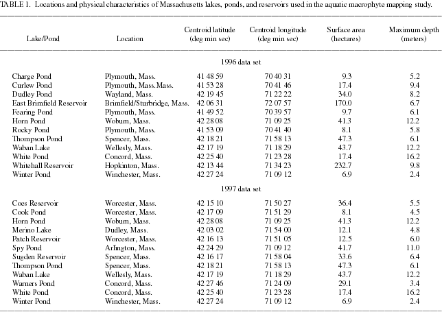
During 1996-98, distributions of floating, emergent, and submersed aquatic macrophytes were mapped in 44 Massachusetts lakes, ponds, and reservoirs by USGS and DEM staff and by volunteers affiliated with the MassWWP. Twenty-four sets of maps, 12 produced in 1996 and 12 produced in 1997 from 19 of the lakes, were used to develop the TM-based mapping procedure. Excessive cloud cover during mid-to-late summer 1998 precluded the use of maps produced in that year. The lakes are primarily in the eastern half of Massachusetts and represent the range of lake types in that part of the State. Locations and physical characteristics of the lakes are presented in Table 1. Surface areas of the lakes ranged from 6.9 to 232.7 ha with a median surface area of 29.1 ha. Maximum depths ranged from 2.4 to 16.2 m (meters) with a median depth of 6.1 m.

Participants in the data-collection effort received training in field-mapping procedures. Mapping was conducted once each summer after the aquatic plants reached their maximum densities but before they began to senesce in early autumn. For each lake, a set of blank maps (field maps) was produced with a 1:24,000-scale (USGS Digital Line Graphs) outline of the lakeshore overlain by a lattice of cells representing the 30-by-30-m spatial resolution of the TM images. These field maps were used by observers to record the macrophyte distributions.

Aquatic plant beds were identified and mapped separately as floating, emergent, or submersed growth forms. Floating aquatic plants (e.g., water lillies [Nuphar sp., Nymphaea sp.] and water shield [Brasenia Schreberi]) commonly are found from the shoreline inward to depths of between 1 and 3 m. They may or may not be rooted in the sediments. Emergent plants (e.g., cattails [Typha sp.], grasses [Phragmites sp.], rushes [Juncus sp.], sedges [Scirpus sp.], arrow arum [Peltandra virginica], and pickerelweed [Pontederia cordata]) typically are rooted and have foliage that extends out of the water. Emergent plants generally are found along the edges of lakes in shallow water rarely exceeding 1 m in depth. Submersed plants (e.g., fanwort [Cabomba sp.], various pondweeds [Potamogeton sp., Najas sp.], coontail [Ceratophyllum sp.], watermilfoil [Myriophyllum sp.], and bladderwort [Utricularia sp.]) may occur from the shoreline across the entire lake bottom, but rarely extend beyond a depth of 10 m because of hydrostatic pressure and the limited penetration of underwater light.

Mapping of floating and emergent aquatic macrophytes consisted of moving slowly along the shoreline in a boat and recording the locations of the plant beds on the field maps. The lattice of 30-by-30 m cells superimposed on the lakeshore outline provided a scale by which observers could judge distances from the shore and accurately mark locations of the beds. The maps also indicated the positions of major landmarks such as roads, dams, and tributary streams and these provided addtional reference points for mapping. Plant density within the mapped beds was estimated by the observers as (1) open water, (2) sparse (greater than 0 but less than 25 percent cover), (3) moderate (greater than 25 percent but less than 50 percent cover), (4) dense (greater than 50 percent but less than 75 percent cover), (5) very dense (greater than 75 percent cover but less than 100 percent cover), or (6) complete (100 percent cover). Visual comparison of duplicate maps prepared at the same time by independent observers for three lakes in 1998 indicated that these density ranges were large enough to subsume minor differences or errors in the observers' density estimates.

Mapping of submersed aquatic macrophytes consisted of establishing multiple transects extending from shore to shore across the lakes. Landmarks represented on the maps were used as control points in locating the transects. Sampling points were then located at intervals of 60 to 120 m along each transect, either by direct measurement with a range finder or by estimating the distance and marking the position relative to the 30-by-30-m cells printed on the map. At each sampling point, a weighted two-sided rake, 46-cm (centimeters) in length, was lowered on a line and dragged along the lake bottom for a distance of about 2 m. The relative amount of plant material retrieved on the rake was used to estimate the areal coverage of submersed aquatic plants at that point. A submersed-vegetation distribution map was then produced for each lake based on the estimated areal coverages.

Image processing using GIS

The hand-drawn distribution maps were digitized by scoring the centroid of each 30-by-30-m cell as one of the six ranges of cover values, based on the mapped locations of the macrophyte beds. The scores for each map were then used to populate the cells of a raster grid corresponding to the lattice originally plotted on the map. The resulting grids were vectorized, clipped into the lake shoreline boundaries, and merged into a single data layer for each vegetation-cover type. The three data layers were then merged into a single data layer maintaining the cover values for each vegetation-cover type.

Because the emergent vegetation was always distributed close to the lake shorelines, and because it represented only a small part of the total covered area of most lakes, the cover values for floating and emergent vegetation types were combined into a single surface vegetation type. Also, the six original vegetation-cover classes were reduced to four summary classes--(1) open water, (2) 1-50 percent surface vegetation cover, (3) 51-100 percent surface vegetation cover, and (4) submersed vegetation at all densities--when preliminary analyses indicated a potential bias in favor of open water. The result of combining vegetation-cover classes with small areal distributions into larger summary cover classes was to reduce the influence of the large areal extent of open water in many of the field maps on the final assignments of the TM pixel-brightness values.

TM scenes acquired by Landsat 5 in July 1996 and August 1997 were obtained from the USGS Earth Resources Observation Systems (EROS) Data Center (EDC). Each scene is comprised of pixels representing either 30-by-30-m (for visible and reflected-infrared (IR) wave bands) or 120-by-120-m (for the thermal-IR wave band) ground-resolution cells. This study used data from visible TM wave bands 2 (TM2, 0.52-0.60 mm [micrometer]) and 3 (TM3, 0.63-0.69 mm), and reflected-IR wave band 4 (TM4, 0.76-0.90 mm). Data for each pixel consist of digital numbers (DNs) ranging from 1 to 255 representing the recorded intensity of reflected radiation in one of the wave bands. The scenes were radiometrically and geometrically corrected, rotated, and aligned to state plane coordinates by the EDC.

Data in the TM scenes were processed into ARC/INFO by creating raster grids for TM2, TM3, and TM4 DNs. Grids for individual lakes were generated from these four TM scene raster grids and rectified to the lake grids. The individual lake grids were then vectorized, clipped into the lakeshore boundaries, and merged into a single data layer for each of the three TM bands. The three data layers were then merged into a single data layer maintaining the DNs for each TM band. The effects of atmospheric haze were removed from the data for TM2 and TM3 by subtracting the smallest DNs for each wave band from all the brightness values for that wave band in the vector grid (Wilkie and Finn, 1996).

Image interpretation using GIS

For each 30-by-30-m cell in the data layer, a normalized difference vegetation index (NDVI; Lillesand and Kiefer, 1994) was calculated using the haze-corrected DNs for TM3 and TM4 as follows:

This data layer was merged with the data layer containing the four vegetation-cover classes. Inconsistencies in alignment of the 30-by-30-m cells in the two data layers were corrected by bringing the combined data layer back into raster grid mode and using coordinates for each lake derived from the original TM images to rectify the cells in the vegetation-cover class data layer. The combined data layer was vectorized and 30-by-30-m cells falling entirely within lakeshore boundaries were given a new attribute that differentiated them from the smaller cells that intersected the shorelines. Cells associated with islands in the lakes were similarly differentiated.

Cells that did not intersect with lake shorelines were grouped according to their NDVI values. For each NDVI value, the total areas were determined for the two surface vegetation-cover classes (1-50 percent and 51-100 percent floating and emergent) and for a hybrid vegetation-cover class consisting of open water and submersed vegetation. The vegetation-cover class comprising the largest total area of the three was then assigned to that NDVI value. In this way, each NDVI value was associated with either a surface-vegetation cover class or with open water. The results were then expanded to the shore cells using the NDVI values as a relate.

The vegetation-cover class assignments for each cell were then examined to determine if any should be changed based on the NDVI values of adjacent cells. If a given NDVI value predominated in the eight-cell neighborhood surrounding a cell, then that NDVI value was added to the cell as an alternative value. Next, all cells with that combination of NDVI value and alternative value were selected and assigned the vegetation-cover class most frequently associated with the combination. In this way, some inconsistent assignments arising from the limited spatial resolution of the TM data were removed.

To determine areas of submersed vegetation, all cells that were not assigned a surface-vegetation cover class in the NDVI analysis were isolated, and a ratio index was calculated by dividing the haze-corrected DNs for TM2 by those for TM3. The steps performed to assign NDVI values were then repeated on these isolated cells, the one difference being that the cells digitized as submersed vegetation were maintained and included as an option for assignment.

Results

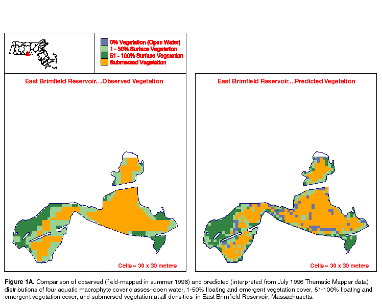
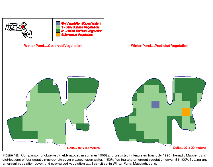
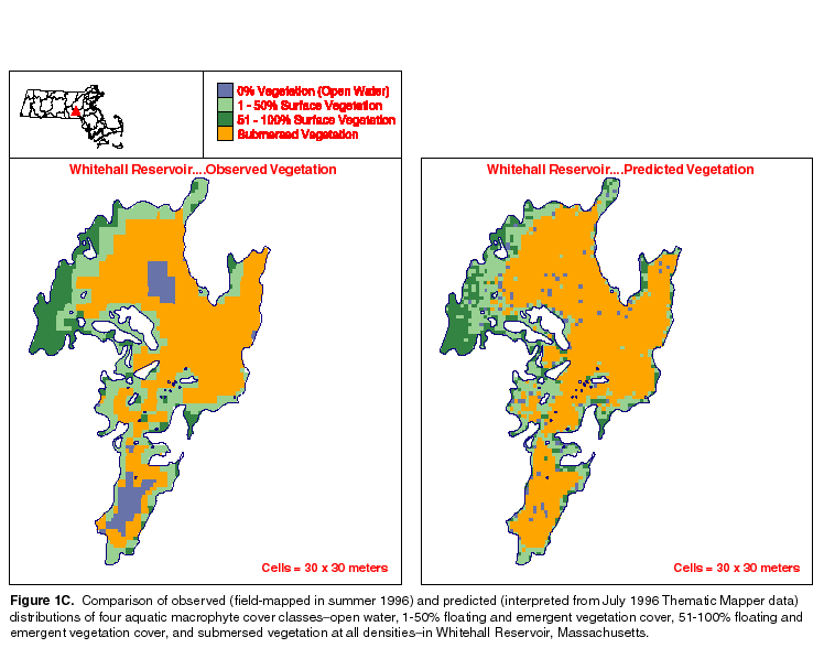
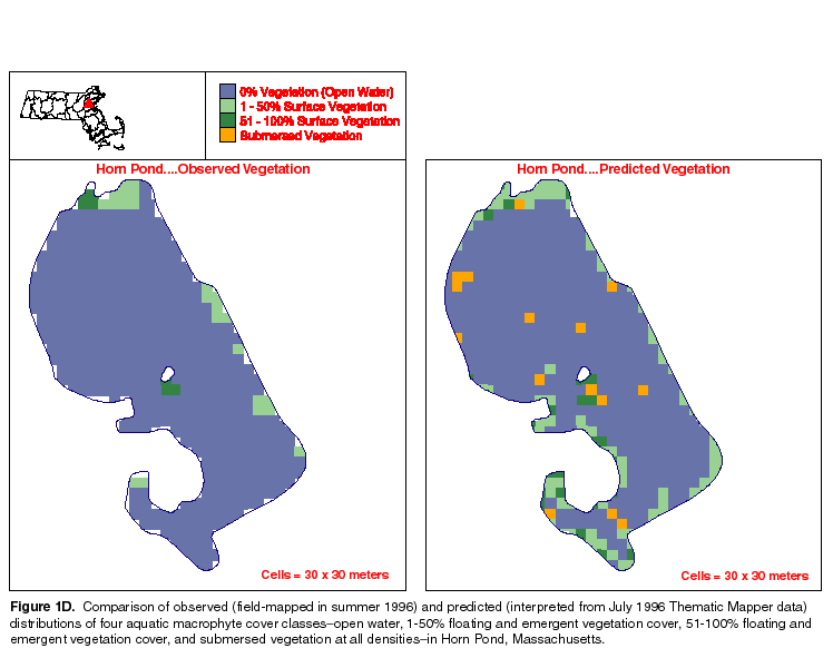
The analysis was performed separately on the 1996 and 1997 data sets, and the resulting TM-based maps were compared with the original digitized field maps. Observed and TM-based distribution maps for four lakes from the 1996 data set are shown in figures 1A, 1B, 1C, and 1D. Agreement between observed and predicted distributions of the four vegetation-cover classes was equally good for lakes with surface areas ranging from 6.9 (fig. 1B) to more than 232 ha (fig. 1C).

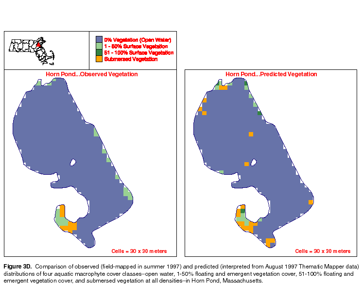
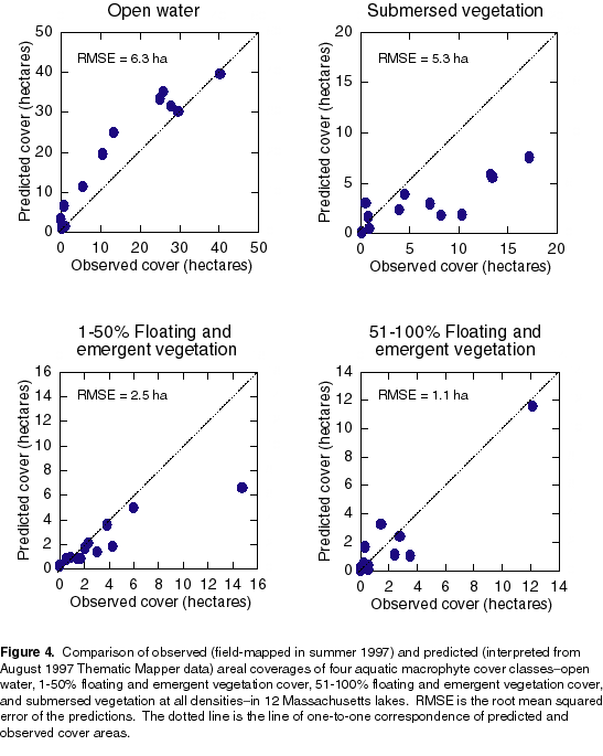
In figure 2, the relation between observed and predicted cover areas is shown for all 12 1996 study lakes for each of the four vegetation-cover classes. For open water, the root-mean-squared-error (RMSE) of the prediction was 3.6 ha for observed cover areas ranging from 0 to 39.7 ha. Predicted open-water cover areas tended to be smaller than observed open-water cover areas. This effect can been seen in figure 1C, for Whitehall Reservoir, and figure 1D, for Horn Pond, where several open-water cells along the lake margins were interpreted as floating or emergent-plant cells and other mid-lake open-water cells were interpreted as submerged. Agreement between observed and predicted cover areas for the other three vegetation-cover classes was very good, with RMSE ranging from 1.3 ha for 51-100 percent floating and emergent vegetation cover to 5.7 ha for submersed vegetation cover.

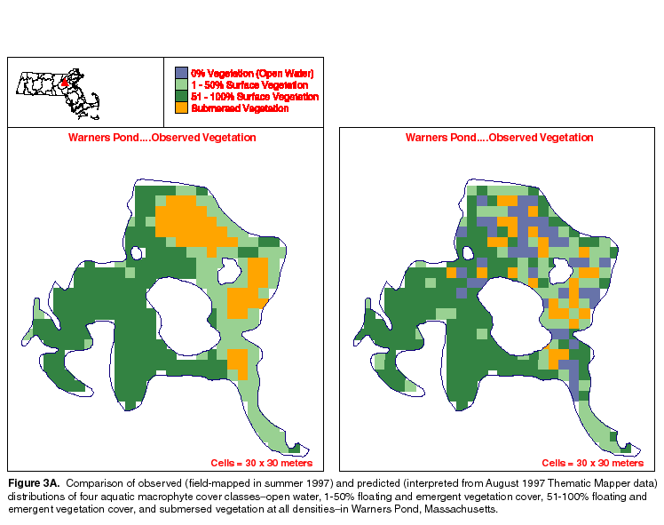
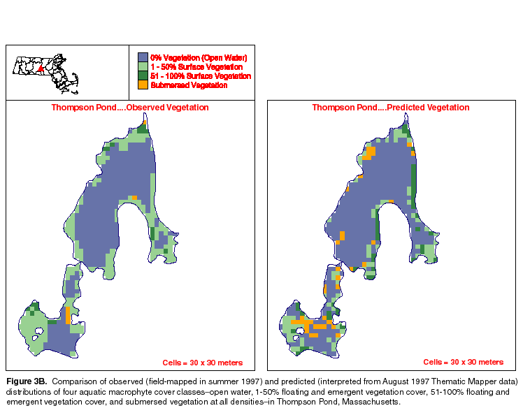
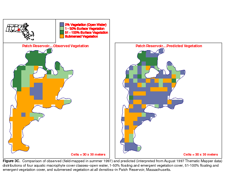
The TM-based maps developed from the 1997 data set did not match the observed maps as closely as did those developed from the 1996 data set (figs. 3A, 3B, 3C, and 3D). The TM-based mapping procedure predicted larger amounts of open-water cover area and smaller amounts of submersed vegetation cover area than were observed (fig. 4), although the RMSE values were similar to those exhibited by the 1996 relations (6.3 ha for open-water cover and 5.3 ha for submersed vegetation cover). Lakes in the 1997 data set tended to have larger observed open-water cover areas than those in the 1996 data set. The median observed open-water cover area was 11.9 ha in the 1997 data set and 8.2 ha in the 1996 data set. Similarly, observed cover areas for submersed vegetation were much smaller in the 1997 data set (median = 0.7 ha) than they were in the 1996 data set (median = 5.8 ha).

Agreement between observed and predicted cover areas was better for the two floating and emergent vegetation-cover classes (the RMSE was 2.5 ha for the 1-50 percent floating and emergent cover class and 1.1 ha for the 51-100 percent floating and emergent cover class) than it was for the open water and submersed-vegetation cover classes (fig. 4). Because most of the observed areas for these classes were very small (1 to 6 ha), however, the errors are significant.

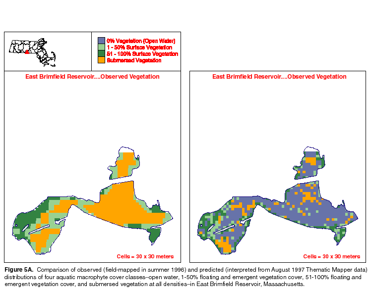
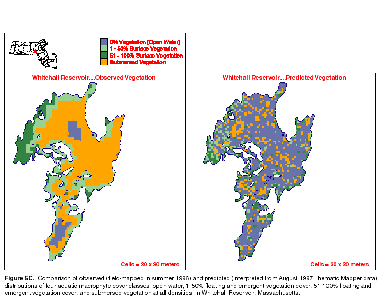
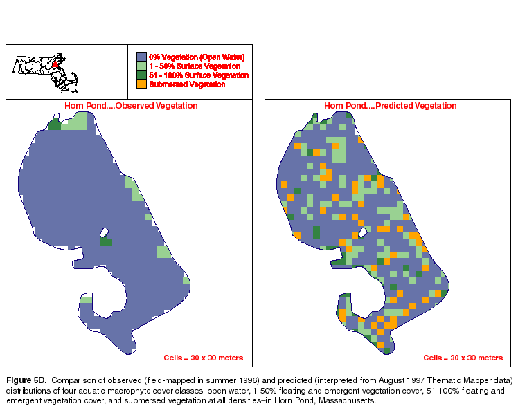
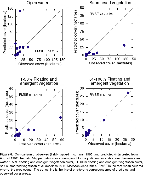
An attempt to predict vegetation-cover class areas in the 1996 study lakes based on interpretations developed from the 1997 data set was unsuccessful. Large areas of submersed or floating and emergent vegetation were interpreted in many lakes as open water (figs. 5A, 5B, 5C, and 5D). Consequently, predicted cover areas for submersed vegetation and 1-50 percent floating and emergent vegetation were smaller than the corresponding observed cover areas and had correspondingly large RMSE values (27.7 ha and 11.4 ha, respectively [fig. 6]). The only exceptions were the predictions for the 51-100 percent floating and emergent cover areas, which produced a RMSE of 1.1 ha over observed (1996) cover values ranging from 0 to 26.8 ha.

Discussion

These results demonstrate that Landsat TM imagery analyzed through a GIS can be used to map distributions of broad classes of aquatic macrophytes in inland waters typical of eastern Massachusetts, provided that suitable field data are available to calibrate the image interpretation. Predicted sizes of open-water, submersed, and floating-and-emergent cover areas closely matched observed sizes in a set of field observations and corresponding TM images acquired in the summer of 1996. Agreement between observed and predicted 1996 submersed-plant cover areas was at least as good as the 56- to 70-percent accuracy reported for mapping studies using visual interpretations of aerial photographs (Schloesser et al., 1987); however, the same analysis applied to a set of data acquired in the summer of 1997 resulted in somewhat less reliable predictions, and an attempt to predict 1996 vegetation-cover areas using the relations developed in the 1997 analysis was unsuccessful.

Differences in the predictive power of the two data sets appear to stem from differences in the relative sizes of the vegetation-cover areas used in the initial calibration of the NDVI values. The ranges of observed areas of the four vegetation-cover classes were similar in the 1996 data set. By contrast, open water predominated in lakes forming the 1997 data set, and the other vegetation-cover classes had much smaller and more variable ranges. Both the field-mapping and the TM-imaging processes are subject to error. Locations of the plant beds indicated on the field maps cannot be exact, and the TM images are limited by the 30-by-30-m ground resolution of the instrument. Under these conditions, a preponderance of one type of vegetation cover class in the calibration data set is likely to result in more assignments of NDVI values to that cover class, simply because locational errors involving that cover class will tend to occur more frequently. It is also possible that the failure of the method to accurately predict the 1996 macrophyte distributions based on interpretations of 1997 data was due in part to this problem.

Ideally, the method should be applied to a set of mapped lakes and then tested on a second set not used in the initial calibration. This was not possible given the limited number of field maps available in the two data sets and the need for equal areal representation of vegetation-cover classes. By careful selection of the initial set of lakes to ensure adequate representation of vegetation cover, it may be possible to use fewer lakes in the calibration process without sacrificing predictive power. The calibration data set also could be improved by using a global-positioning system to accurately locate and map the aquatic plant beds.

With these modifications, it should be possible to use TM imagery to develop macrophyte maps for most of the 3,000 named lakes, ponds, and reservoirs in Massachusetts. A statewide mapping effort would require the purchase of at most three TM scenes. Each scene would require a calibration data set consisting of 10 to 15 mapped macrophyte distributions. These data could be collected by two individuals in 15 to 20 working days, depending on the surface areas of the largest lakes. Digitization of the field maps and image interpretation could be accomplished by one individual, familiar with both macrophyte ecology and ARC/INFO, in another 15 to 20 working days. The resulting areal distributions could then be used for statewide assessments of lake quality and trophic state, and for monitoring long-term trends in lake eutrophication.

Acknowledgments

The authors wish to thank the volunteers and staff of the Massachusetts Water Watch Partnership for their generous contributions of time and other resources to this project. Bruce E. Taggart, Curtis V. Price, Paul K. Barten, and Barbara A. Korzendorfer read earlier versions of the manuscript and provided many helpful comments and criticisms.

References cited

Canfield, D.E., Jr., Langland, K.A., Maceina, M.J., Haller, W.T., and Shireman, J.V., 1983, Trophic state classification of lakes with aquatic macrophytes: Canadian Journal of Fisheries and Aquatic Sciences, v. 40, p. 1713-1718.

Lillesand, T.M., and Kiefer, R.W., 1994, Remote sensing and image interpretation, 3rd ed.: New York, N.Y., John Wiley and Sons, Inc., 750 p.

Marshall, T.R., and Lee, P.F., 1994, Mapping aquatic macrophytes through digital image analysis of aerial photographs: an assessment: Journal of Aquatic Plant Management, v. 32, p. 61-66.

Massachusetts Water Resources Commission, 1994, Policy on lake and pond management: Boston, Mass., Masschusetts Water Resources Commission, Div. of Water Resources, 5 p.

Schloesser, D.W., Manny, B.A., Brown, C.L., and Jaworski, E., 1987, Use of low-altitude aerial photography to identify submersed aquatic macrophytes, in Color Aerial Photography in the Plant Sciences and Related Fields: Ann Arbor, University of Michigan, Proceedings of the 10th Biennial Workshop (1984), p. 19-28.

Wilkie, D.S., and Finn, J.T., 1996, Remote sensing imagery for natural resources monitoring--A guide for first-time users: New York, N.Y., Columbia University Press, 295 p.

Author information