Hydrologic Model of the Buffalo Bayou Using GIS
James H. Doan, P.E.
US Army Corps of Engineers � Hydrologic Engineering Center
Davis, California
Abstract
The hydrologic model of the Buffalo Bayou Watershed was simulated using the Hydrologic Modeling System with inputs derived from the Geographic Information System. The Buffalo Bayou Watershed covers most of the Houston metropolitan area in Texas. The watersheds and streams were delineated from the USGS digital elevation models (DEM) at 30-meter cell resolution and stream data from USGS digital line graph (DLG) and EPA river reach file (RF1). Physical watershed parameters were extracted from the CRWR-PrePro program to support hydrologic parameters computation. The model uses ModClark runoff transformation with grid-based NEXRAD radar rainfall .
The first recorded flood in 1929 in the Buffalo Bayou watershed devastated the Houston, Texas. Since then, other flooding events followed in similar vigor and intensity. Local governments have been actively dealing with floods by building dams and reservoirs to regulate flows to downstream Buffalo Bayou Creek. With the low-relief terrain in the watershed, local governments have also enhanced the conveyance capacity by improving streams by straightening reaches, lining channel, and installing hydraulic structures. Although these flood control measures have brought many benefits, the existing flood control infrastructure has been increasingly burdened due to significant urbanization in recent years. Coupling the tremendous growth in Houston with the potential for a large rainfall event similar in magnitude to the 43 inches in a 24-hour period storm recorded at nearby Alvin, Texas, the rising concerns over flooding is warranted. To safeguard from future flooding, the Galveston District of the US Army Corps of Engineer has funded this project as a first step towards achieving the long-term goal of developing a Water Control Data System (WCDS). The WCDS will offer real-time monitoring, active warning, and forecasting of floods in the region as shown in Figure 1.
Figure 1: Buffalo Bayou Watershed, Houston, Texas
The Buffalo Bayou project meets many of the long-term objectives for developing a WCDS. The first objective is to develop a hydrologic modeling using Hydrologic Modeling System (HMS) for the study area upstream of the Piney Point streamflow gage located on the Buffalo Bayou Creek downstream of the dams. The HMS model of the Buffalo Bayou watershed will employ a quasi-distributed rainfall to runoff transformation procedure called Modified Clark (ModClark) and grid-based NEXRAD radar rainfall in the Standard Hydrologic Grid (SHG) format to model the watershed response to the storm event in October 16-18, 1994. The second objective is to develop, maintain, and use the GIS spatial database of thematic layers to generate inputs for HMS, visualize data, and document watershed conditions.
The Galveston District of USACE contracted HEC to develop a hydrologic model using HEC-HMS. The HEC-HMS model will include a basin, precipitation, and control specifications model in accordance to the following guidelines.
Basin Model
Precipitation Model
Control Specifications Model
This Buffalo Bayou project has exposed numerous benefits gained through integrating GIS technology to solve water resources issues. These benefits will lead to improve modeling techniques for studying the watershed and its conveyance system, expedient extraction of watershed parameters, accurate visualization and documentation of the watershed infrastructures and conditions, and effective communication tools. The management people responsible for uncovering these benefits by providing funds, visions, and supervisions are Charles Scheffler - Chief of the Hydrology and Hydraulic Branch at Galveston District of the US Army Corps of Engineers, Arlen Feldman - Chief of the Research Division at HEC, Darryl W. Davis - Director of HEC, and David Maidment - Director of Center for Research in Water Resources (CRWR) at the University of Texas at Austin.
The expertise and valuable contributions offered by Seth Ahrens of the Center for Research for Water Resources of University of Texas at Austin and Harris County Flood Control District are greatly appreciated.
Literature Review and GIS Supplemental Background Information
The watershed description and its conveyance system have been distilled from previous project reports, correspondence with Galveston District and HCFCD, hydrologic models, and watershed delineation maps. While the literature review was helpful, field observations conducted on May 16 and October 12, 1998 provided many clarifications on the stream networks and their drainage facilities. The information gathered from field observations have been geographically referenced and incorporated in the GIS spatial database for visualization and documentation. The GIS spatial database supported overlays of aerial photography with streams and gage locations, providing valuable supplemental information.
Watershed Description and Conveyance System
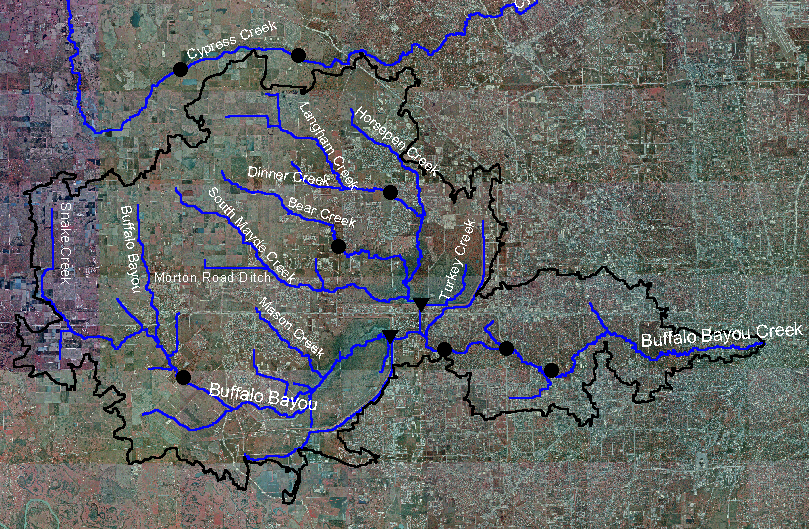
The Buffalo Bayou watershed is approximately 341 square miles and lies primarily in Harris and Fort Bend Counties in southeast Texas. The Buffalo Bayou watershed generally consists of two major drainage areas: the Addicks and Barker Reservoir watershed as shown in Figure 2. In moderate to larger storm events, however, the Buffalo Bayou watershed also drains portions of the Cypress Creek watershed that overflow south into the Addicks Reservoir watershed. The excess rainfall over the Buffalo Bayou watershed is conveyed slowly over the low relief landscape. When it enters the streams, it often travels through a series of hydraulic structures through the urban area before it can exit through the electronically controlled conduits installed in the Addicks and Barker reservoirs. Primarily for flood control, the Addicks and Barker Dam form detention reservoirs that have been used to regulate flow releases downstream into the Buffalo Bayou Creek electronically. Downstream of both dams, the Buffalo Bayou Creek�s non-damaging capacity has been established to be 2000 cfs. The drainage area downstream of the dams is referred to as Buffalo Bayou Local. The Buffalo Bayou Creek then flows through the Houston Ship Channel for about 32 miles and becomes a tributary of the San Jacinto River. From a land-use perspective, the condition of the Buffalo Bayou watershed was undeveloped as of 1977. In contrast, the tremendous growth rate of the Houston area is extending suburban development into these watersheds in recent years.
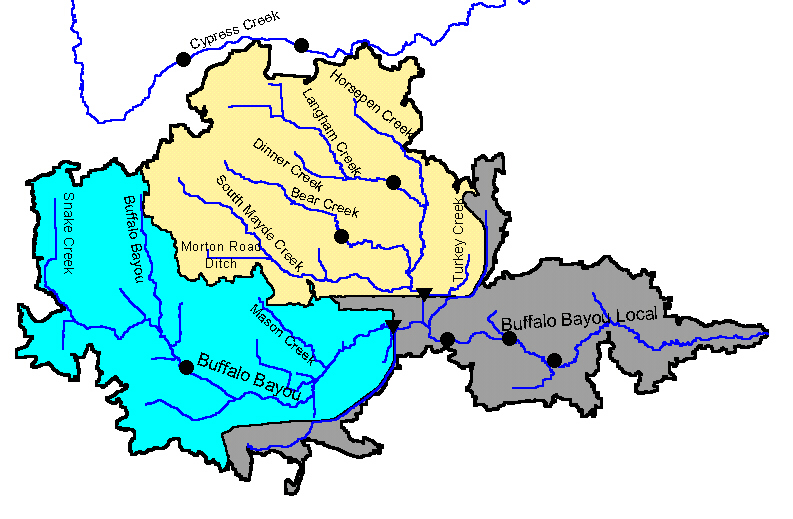
Figure 2: Buffalo Bayou Watershed
The Addicks Reservoir watershed of about 134.4 square miles lies mostly within Harris County and a small area of about 18 acres lies within Waller County. The watershed slopes about 0.10% from northwest to the southeast. Ground elevations vary from163 feet mean sea level (msl) with the 1973 adjustment along northwestern boundary of the watershed to 71.1 feel msl at Addicks Dam. The mean annual rainfall is 45.75 per year. The soil type is classified as Hydrologic Soil Group D, which has high runoff potential and very slow infiltration rates. The runoff generally travels slowly overland due to mild slope, collects in streams, accumulates in the Addicks reservoir, and discharges through electronically controlled gated conduits into Buffalo Bayou Creek. The following streams and the drainage areas have been identified for the study as shown in Table 1.
Table 1: Major Streams in the Addicks Reservoir Watershed
|
Major Streams |
Drainage Area (sq.mi.) |
|
South Mayde Creek |
31.0 |
|
Bear Creek |
22.9 |
|
Langham Creek |
36.8 |
|
Dinner Creek |
8.2 |
|
Horsepen Creek |
19.5 |
|
Turkey Creek |
7.4 |
|
Ditch Along Morton Road |
8.6 |
Buffalo Bayou watershed above Barker Dam lies within Harris, Waller, and Fort Bend Counties. The watershed is about 124.5 square miles. Natural ground elevations vary from 200 feet msl at the upstream divide to about 73 feet msl at Barker Dam. Natural streamflow gradients in the basin are uniform at about 5 feet per mile sloping in a southerly direction. When a rainfall event occurr, the runoff travels slowly overland due to mild slope, collects in streams, accumulates in the Barker reservoir, and discharges electronically through gated conduits into Buffalo Bayou Creek.
The Barker Dam was designed and constructed solely for flood control purposes in 1945 by the US Army Corps of Engineers. Both the Addicks Dam and the Barker Dam consists of long earthen embankments with five gated conduits capable of discharging floodwaters into downstream channels. The following streams and the drainage areas have been identified for the study as shown in Table 2.
Table 2: Major Streams in the Barker Reservoir Watershed
|
Major Streams |
Drainage Area (sq.mi.) |
|
Buffalo Bayou Creek |
78.6 |
|
Mason Creek |
9.4 |
|
Snake Creek |
36.5 |
The Cypress Creek watershed of about 130 square miles lies to the north, adjacent to the Addicks Reservoir watershed as shown in Figure 9. The Cypress Creek channel flows easterly to its confluence with the San Jacinto River in Harris County. Only a few feet higher than the stream bank, the shallow Cypress Creek�s flood plain has poorly defined watershed boundaries. Therefore floodwaters from moderate to large rainfall events overflow southward across the divide at multiple locations into the South Mayde, Bear, Langham, and Horsepen Creek of the Addicks Reservoir watershed. This overflow is not returned to the Cypress Creek basin.
Downstream of the dams, the Buffalo Bayou local flows are contributed to by a significant drainage area of 82.1 square miles as shown in Figure 10.
The HMS development has been focuses on building the GIS spatial database with required thematic layers for modeling the terrain and supporting watershed parameters extraction. Programs in ArcInfo, ArcView, DSS, and other utilities are identified and used to develop inputs for HMS. These inputs are brought into HMS, which performs the hydrologic modeling and computes flows at locations of interest to the projects. The software packages used in this study are summarized in Table 3 .
Table 3: Summary of Software Packages
|
HMS |
The Hydrologic Modeling System (HMS) was designed as part of the US Army Corps of Engineers Hydrologic Engineering Center�s (HEC) "Next Generation (NexGen) Software Development Project." With an improved graphics-user interface and advanced technical capabilities for rainfall-runoff processes, HMS will replace the commonly used HEC-1. An HMS model contains three data sets - the basin, precipitation, and control specifications file. The basin file contains hydrologic elements, parameters, and their connectivity to the drainage network. The precipitation file contains meteorological data and methods for averaging the data over the subbasin. The control specifications file identifies the time window of the analysis and computational time interval for the simulation. HMS also employs Data Storage System (DSS) for storage and retrieval of time series and grid-based data and parameters, such as NEXRAD rainfall data and snowmelt and soils moisture accounting parameters. |
|
Arc/Info |
Version 7.2.1 or later from Esri was used for grid data (DEM) assembly and grid projection to SHG rainfall grid type. |
|
ArcView |
Version 3.1 or later from Esri with Spatial Analyst Extension 1.1 and 3D Analyst 1.0. ArcView serves as the foundation for most of the GIS terrain analysis, data visualization, and documentation. |
|
CRWR-PrePro |
CRWR-PrePro version 3.0 from CRWR is a system of scripts and associated tools that runs within ArcView with Spatial Analyst Extension. Using the grid-based terrain model built from the DEM, CRWR-PrePro delineates streams and watersheds, determines their interconnectivity, and calculates many physical and hydrologic parameters. CRWR-PrePro prepares an ASCII file in HMS basin format for transferring GIS results into HMS. |
|
GridParm in Arc/info |
GridParm is implemented as a system of Arc/Info macros that derive a grid cell-parameter file required by the ModClark quasi-distributed method of simulating basin runoff with radar rainfall measurements. The cell-parameter file consists of hydrologic properties of cells defined by the intersection of watershed boundaries with a precipitation-reporting grid in either the National Weather Service�s Hydrologic Rainfall Analysis Project (HRAP) grid or the Standard Hydrologic Grid (SHG). Currently, the cell-parameter file contains the following parameters.
The cell-parameter file has been expanded to meet new parameter requirements, such as grid-based curve number and snowmelt parameters. As an example, SCSParm is another ArcInfo program that works in conjunction with GridParm to extends cell-parameter file to include curve numbers at the cell level. |
|
ModClark Implementation in ArcView |
A prototype version of ModClark procedures has been developed in ArcView during this project. |
|
Data Storage System |
Data Storage System (DSS) is used for storing, retrieving, and accessing long periods of time-series data, such as streamflow and point precipitation. In this project, a specialized DSS was used to store grid-based radar rainfall. A utility, Ascii2DSS, was used to bring slices of radar rainfall into DSS every 5 minutes. The DSS stores over 300 radar scenes of the October 16-18, 1994 storm over the entire study area. |
The roles of the GIS include terrain analysis, data visualization and exploration, and project documentation. Fulfilling these roles requires that all thematic layers be in the same coordinate system and projection. The selected projection coincides with the SHG projection as described in Table 4. Based on the Albers Equal Area, the SHG projection offers many advantages in hydrologic modeling, such as uniform volume of water on a cell basis.
Table 4: Standard Hydrologic Grid Definition
|
Units |
Meters |
|
Datum |
North American Datum, 1983 (NAD83) |
|
1st Standard Parallel |
29 degrees 30 minutes 0 seconds North |
|
2nd Standard Parallel |
45 degrees 30 minutes 0 seconds North |
|
Central Meridian |
96 degrees 0 minutes 0 seconds West |
|
Latitude of Origin |
23 degrees 0 minutes 0 seconds North |
|
False Easting |
0.0 |
|
False Northing |
0.0 |
Once the GIS data sets are organized in the proper coordinate system and projection, modeling a topographically driven flow network can be performed with the GIS procedures. More importantly, these GIS procedures can prepare HMS inputs, such as the basin, precipitation, and ModClark files, which are time-consuming, inconsistent, and error-prone if prepared by manual methods. Therefore, GIS software has evolved to contain hydrologic functions.
The compilation of GIS data sets require conversions of file format, coordinate systems, as well as geographical referencing of non-spatial data sets. The file are converted to the industry-standard shapefiles format for vector data and Esri�s grid format for raster data. The Esri�s grid format can be used interchangeably between ArcInfo and ArcView. Triangulated Irregular Network (TIN) is Esri�s standard format for the 3D Analyst Extension in ArcView. Examples of vector data that require conversions are Digital Line Graphs for streams alignment and State Soil Geographic Data Base (STATSGO) data for the hydrologic soil types. Examples of raster data that require conversion are DEM, NEXRAD radar rainfall, and curve number grid. A TIN can also created to represent the terrain.
It is important to note that these data sets have been re-projected into the SHG projection to insure that all data sets in vector, raster, and TIN are in proper alignment and refer to the same ground surface. For example, originally in the Universal Transverse Mercator (UTM) projection, the DEM was re-projected into the SHG projection; non-spatial data sets, such as aerial image and streamflow gage, were geographically reference to the SHG. Most of the information was acquired online through government�s web sites on the Internet as shown in Table 5. A few data sources such as NEXRAD rainfall and the SHG curve number grid were obtained from local authorities and academia. The GIS data development for the study area includes all of Buffalo Bayou watershed, downtown Houston, and most of greater metropolitan Houston.
Table 5: GIS Spatial Database - Data and Sources
|
Data Types |
Description |
Source |
|
Digital Elevation Model (DEM) |
Originally converted from USGS 7.5-minute quads, the DEM data at 30- by 30-meter resolution is available for the study region from the Texas Natural Resources Information System (TNRIS). |
www.tnris.state.tx.us |
|
Spatial Rainfall Data |
Radar rainfall (NEXRAD Stage III) has been compiled for a severe storm event during 16-18 October 1994. At one square kilometer resolution, rainfall intensities are available approximately every six minutes. The rainfall intensity has units of mm/hr. |
Mary Lynn Baeck and Jim Smith from the Princeton Environmental Institute |
|
Soil Type Data |
Soil type data under Soil Surveys Geographic Data Base (SSURGO) data is very limited in the study region. Therefore, soil type data under STATSGO data has been selected for the study. The data was collected from 1- by 2-degree topographic quadrangle maps. |
United States Department of Agriculture STATSGO CD- ROM |
|
Digital Line Graph (DLG) Data |
Digital Line Graph data is available at 1:100,000 scale from the United States Geological Survey (USGS). This data was derived from 1:100,000 scale, 30- by 60-minute quadrangle USGS maps. The data exists as DLG level-3 format. |
edcwww.cr.usgs.gov |
|
Stream Coverage |
Stream coverage is obtained from the Environmental Protection Agency (EPA) river reach file (RF1). Projected in Albers equal area format, the data has approximate scale of 1:500,000. |
h2O.er.usgs.gov/nsdi/wais/water/rf1.html |
|
Street Coverage |
The Environmental System Research Institute (Esri) has compiled a street database for the entire United States. The data is developed from the Geographic Data Technology�s Dynamap/1000 street database, version 1 dated 1995. This data can be viewed with Esri ArcView software. |
Esri Street Database CD-ROMs. |
|
Land Use/Land Cover |
The land use and land cover data uses the Anderson Land Use Code (Level II) classification system. At 1:250,000 scale and in Universal Transverse Mercator (UTM) projection, the data was derived from the USGS Houston and Beaumont 1- by 2-degree quadrangle maps. This data was downloaded from the Texas Natural Resources Information System (TNRIS). |
nsdi.usgs.gov/nsdi/products/lulc.html |
|
Digital Orthophoto Quarter Quads (DOQQ) |
Digital areal photos at 30-meter resolution were obtained for the study region from the Texas Natural Resources Information System (TNRIS). |
www.tnris.state.tx.us |
|
Streamflow Gage Data |
Streamflow data for Buffalo Bayou watershed for October 1994 at gages maintained by the USGS. |
www.usgs.gov |
|
Curve Number Grid |
Curve number data that is widely accepted by water resources community in Texas. |
CRWR of the University of Texas at Austin |
|
Drainage Facilities Photographs |
Photographs were taken looking upstream and downstream and at faces of accessible drainage structures. |
Field observations on May 16 and October 12, 1998. |
The primary GIS data sets as input to CRWR-Prepro consisted of the DEM, DLG, and streamflow gage locations.
The DEM was converted from the USGS 7.5-minute quad maps. The 48 tiles of DEM were joined together by ArcInfo using the Grid Extensions. The resulting DEM had data gaps along tile edges as shown in Figure 3. The data gaps were filled in with interpolated elevation values from their neighboring cells. After verifying the DEM data against the USGS 7.5-minute quad maps, the complete DEM was used to model the terrain as shown in Figure 4. From correspondence with HCFCD, the DEM data should be unaffected by the subsidence because it occurred to the east of Houston, which is outside of this project area.
The DLG represents water features such as streams, ditches, and drainage facilities in more details than the RF1. Therefore, selective streams and ditches from the DLG�s were imposed on the DEM as a way to compensate for the flat landscape. This process is a way to improve the delineation of streams and subbasins.
During the modeled storm event, the USGS maintained eight flow gages and two reservoir storage gages in the study area. The stream flow gages are located within Harris County. The USGS classifies these stream gages to the Buffalo-San Jacinto Basin with the Hydrologic Unit Code of 12040104. For some of these gages, historical daily peak flow values have been retrieved. Other gages, however, contain annual peak flow values, which do not have the details required for this study.
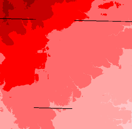
Figure 3: DEM Terrain with Data Gaps
Figure 4: Complete DEM Terrain
Data Visualization and Documentation
The GIS provides good data visualization and documentation support for geographic images, hillshades, and non-spatial data integration. For example, the areal photography in multi-band color DOQQ is used as the background for mapping locations of drainage facilities and stream gages with additional non-spatial data attributes as shown in Figure 5. All of the photographs of drainage facilities taken on May 16 and October 12, 1998 have been geographically referenced in the GIS spatial database. Some areas were not photographed due to road closures, limited access roads, and private property restriction.
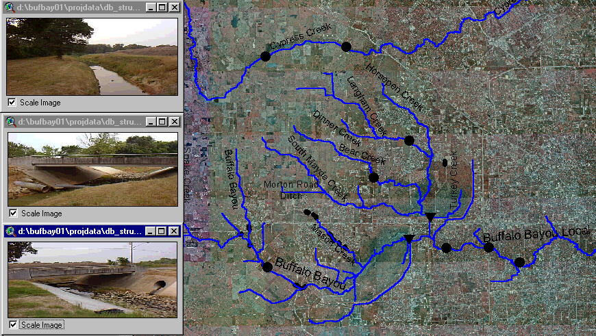
Figure 5: Multi-band DOQQ for Mapping Drainage Facilities
"Hydrologically Corrected" and "Depressionless" Terrain Model
Construction of a "hydrologically corrected" terrain model involves more complexity than combining tiled USSG�s DEMs into a unifying grid. The DEM assembled from the USGS represented by elevation averages at regular intervals may not accurately represents stream locations and watershed boundaries. For example, stream and watershed delineation sometimes does not coincide with published data sources like the EPA�s RF1 and the USGS�s watershed in the Hydrologic Unit Code (HUC). A "hydrologically corrected" terrain model represents accurate flow patterns across landscape, stream alignments, topographic ridges, stream confluences, internal drainage areas, and drainage facilities. Many factors, such as cell resolution, accuracy, topographic relief, and drainage facilities deserve careful considerations because they often affect the quality of the terrain model. In theory, combining GIS data sets of different resolutions is generally not recommended because of the difficulty in assessing the accuracy and the precision of the resulting data set. In practice, however, combining data sets of various resolutions comes out of necessity due to lack of uniform data and data coverage. For example, DLG�s at scale 1:100,000 were imposed on the DEM at 30-meter resolution.
In contrast to the effort required for the "hydrologically corrected" DEM, the "depressionless" DEM is simply constructed by filling in the sinks or depressions in the assembled DEM. Because of the complexity and effort required for constructing a "hydrologically corrected" terrain model, a "depressionless" terrain model often serves as a simpler substitute in the analysis. For study regions with moderate to high topographic relief, the "depressionless" terrain model may be adequate for the analysis. For low-relief regions, however, the "depressionless" terrain model often needs additional work to adequately represent the terrain. For example, the Buffalo Bayou region has undergone many iterations, where drainage ditches, particularly the Morton Road Ditch, and streams were imposed onto the DEM to reach a higher level of hydrologic correctness.
The GIS approaches toward hydrologic analysis requires a terrain model that is "hydrologically corrected". A "depressionless" terrain model is used in the analysis. The GIS analyzes the "depressionless" terrain model by applying the 8-point pour model, where water flows across the landscape from cell to cell based on the direction of the greatest elevation gradient. The process of analyzing the landscape characteristics and slopes for stream networks and subbasin boundaries is presented in Table 6. The steps in the analysis include imposing the streams on the flat terrain, filling depressions or pits, calculating flow direction and flow accumulation, delineating streams with an accumulation threshold, defining outlets from stream segments, adding user-specified outlet location, and delineating the subbasin watershed.
Table 6: GIS Approach Terrain Processes
|
Processes |
Output |
|
Step 1 Depresionless Terrain Fills the terrain pits by increasing the elevation of the pit cells to the level of the surrounding terrain in order to determine flow directions. The pits are often considered as errors in the DEM due to re-sampling and interpolating grid. Elevation unit is in meters. |
|
|
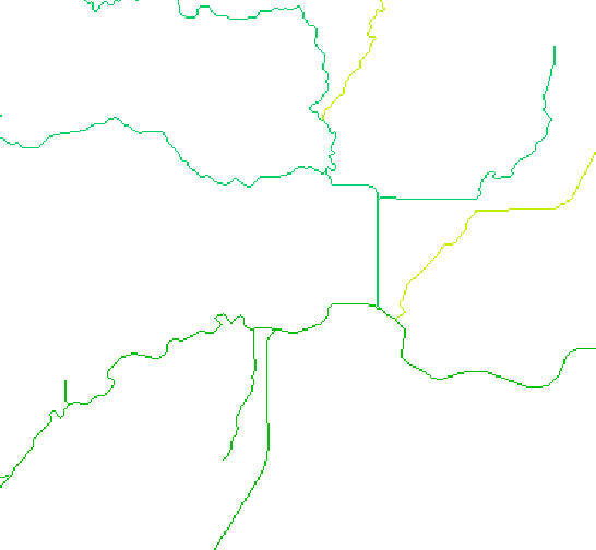
Step 2 Flow Direction Defines the direction of the steepest descent for each terrain cell. Similar to a compass, the 8-point pour algorithm specifies the following eight possible directions: 1 = east, 2= southeast, 4 = south, 8 = southwest, 16= west, 32=northwest, 64 = north, 128=norhteast.
Turkey Creek can be seen flowing south according to the flow direction of 4 (blue cells). |
|
|
Step 3 Flow Accumulation Determines the number of upstream cells flowing into a given cell. Upstream drainage area at a given cell can be calculated by multiplying the flow accumulation value with the cell area. |
|
|
Step 4 Stream Delineation Classifies all cells with flow accumulation greater than the user-defined threshold as cells belonging to a stream network. Typically, cells with high flow accumulation, greater than a user-defined threshold value, are considered part of a stream |
|
|
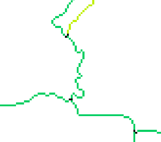
Step 5 Stream Link Stream links or segments are the sections of a stream channel that connects two successive junctions, a junction and an outlet, or a junction and the drainage divide. 215 stream links make up the stream networks.
|
|
|
Step 6 Automatic Outlets Specification Outlets are automatically specified as the most downstream cell of the stream segments. 215 outlets are specified for 215 stream links. |
|
|
Step 7 User-specified Outlet Definition Specifies additional outlets typical of streamflow gages locations and other project control points of interest. |
|
|
Step 8 Watershed Delineation Delineates the areas draining to outlets |
|
One of the strengths of the GIS is the capability to create input files externally that can be imported into HMS. Through spatial analysis, GIS can generate results more efficiently, consistently, and accurately than manual methods. The GIS has produced the basin file, background map file, MoClark�s cell-parameter file, and grid-based NEXRAD radar rainfall data as shown in the following figures.
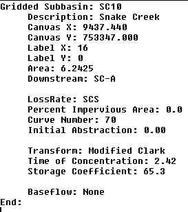
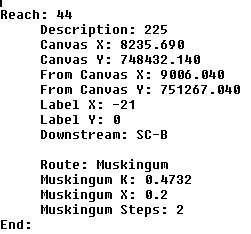
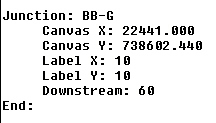
Figure 6: Portions of HMS Basin File in ASCII Format
Portions of the HMS basin files in ASCII format showing the drainage patterns with the subbasins, reaches, and junctions and their respective hydrologic parameters are shown in Figure 6. The basin model shows the hydrologic methods and their applicable loss rates, unit hydrograph, and routing parameters. Some of these hydrologic parameters were inherited from the GIS and not intended to be used in the final HMS model. These hydrologic parameters will be revised within HMS.
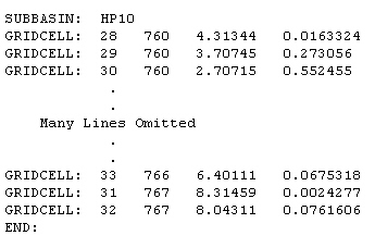
Figure 7: ModClark Cell-Parameter File
The ModClark cell-parameter file showing the X and Y coordinates for SHG cells, their average SHG cell (not DEM cell) travel distances, and areas are shown in Figure 7.
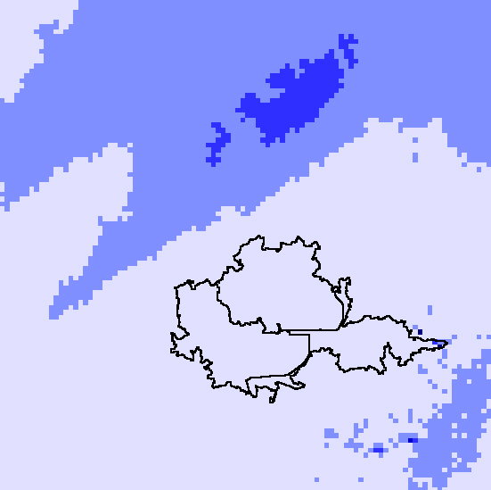
Figure 8: Cumulative NEXRAD Radar Rainfall
The cumulative NEXRAD radar rainfall as shown in Figure 8 is in SHG at 1000-meter resolution. The individual slides of radar rainfall, interpreted for every 5 minutes, shows detailed areal and temporal distribution of rainfall. If the ModClark method is not used, other GIS programs can be used to perform spatial-averages and weights based on Theissen polygons.
The verification of GIS results is an important step before using them in HMS as input. The results were verified by (1) graphically checking against the topographic data, street data and USGS quads, (2) comparing streams and subbasin boundaries with previous HEC-1 model delineation, (3) checking topographic and hydrologic parameters calculations, and (4) comparing drainage area with published information.
Within the GIS spatial database, overlays of pertinent thematic data layers can be viewed simultaneously, facilitating graphical verification. With the subbasin boundaries overlaid on the DEM, the subbasins� shapes and orientations indicates that the flow directions are in agree with the landscape slope. In addition, the capability to zoom aides in clarifying much drainage details, such as the flow of Turkey Creek along the toe of the levee and joins with South Mayde Creek. After checking GIS results with road maps and USGS quad maps, it becomes evident that the Snake Creek basin is a tributary to the Buffalo Bayou and is incorporated into the HMS model. Graphically checking GIS results through data overlays and existing maps comparison can be very useful when previous hydrologic studies are not available.
When previous hydrologic studies are available, however, more detailed verification can be performed by comparing GIS topographic and hydrologic parameters with those of the HEC-1 models. In this project, the combination of 30-meter DEM resolution and low-relief terrain can only support broader subbasin delineation, which covers mostly stream confluences and streamflow gage locations. If DEM is available at finer resolution, more detailed subbasin delineation would be possible; otherwise, attempting to perform more detailed delineation with a 30-meter DEM would likely result in "shaky" or inaccurate subbasin boundaries. Consequently, the subbasins generated from GIS are more generalized and encompass many smaller HEC-1 subbasins; GIS topographic and hydrologic parameters can only be indirectly compared to HEC-1.
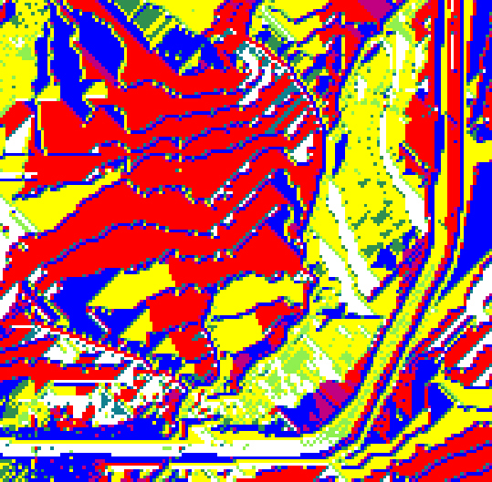
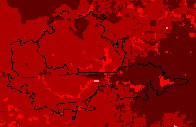
Drainage areas and lumped curve number comparison agree for most subbasins. The SHG curve numbers are within the range of the land uses and soil types in the watershed and generally higher for developed area as shown in Figure 9.
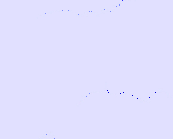
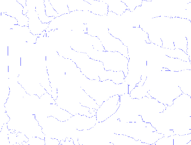
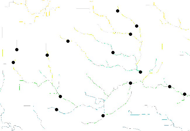
Finally, GIS delineated streams, subbasins, and their associated drainage area were compared with published data sources from the USGS and EPA. For this project, the comparison shows generally good agreement. The GIS delineated streams consistently aligning over with the USGS�s DLG and EPA�s RF1 as shown in Figure 10. At the Piney Point gage on the Buffalo Bayou Creek, it is important to note that the overall drainage area agrees with published information from the USGS.
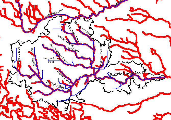
Figure 10: GIS Delineated Streams With The USGS�s DLG and EPA�s RF1
Using GIS as a pre-processor can accelerate the building of an HMS model. The GIS ability can extend beyond processing the terrain model to performing spatially intensive analysis for development of grid-based parameters. The results produced by GIS for HMS can be controlled somewhat by focusing on the GIS�s description of the landscape characteristics and stream networks. From a modeling standpoint, greater control over the model is often necessary to address difficult situations. HMS is powerful in that it offers full control over the model connectivity, methodology, and parameters. For example, HMS can be used to reconfigure the connectivity and eliminate, add, and revise hydrologic elements and their properties. To model the complex Buffalo Bayou conveyance system, it becomes necessary to take advantage of HMS�s flexibility to incorporate the Galveston District�s and HCFCD�s existing hydrologic and hydraulic models in HEC-1 and Water Surface Profiles (HEC-2) as well as modeling the Addicks and Barker Reservoirs. The work going into the three HMS components are discussed below. Some work items are pending because clarifications are required after the Galveston District and the HCFCD have an opportunity to review this report.
The HMS project definition shows the basin, precipitation, and control specification components, which can be selected to create a run as shown in Figure 11.
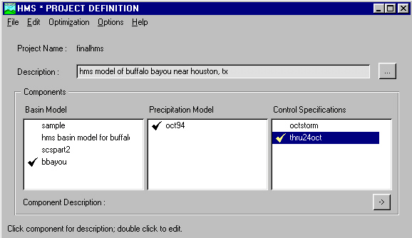
Figure 11: HMS Project Definition
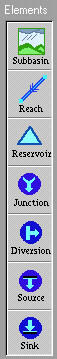
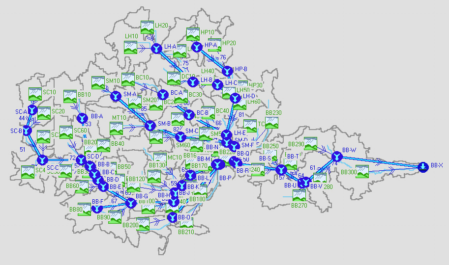
The basin model generated by GIS was imported into HMS as shown in Figure 12. The basin file contains the schematic, hydrologic methods, and their parameters. The basin schematic adequately represents drainage patterns with the connectivity of the hydrologic elements (subbasin, reach, junctions, reservoir, diversion, source, and sink). When the connectivity was checked in detail, the presence of short reaches near stream confluence unnecessarily made the model more complicated and required parameter refinement. HMS can simplify the model and save the effort of parameter refinement by eliminating these short reaches and re-connecting the hydrologic element to the nearby junction downstream. However, this simplification was not necessary since the HMS model can be ran with GIS-generated parameters.
The hydrologic methods and parameters have been created by default methods in GIS. The original intentions were to revise these hydrologic methods and parameters based on existing hydrologic models in HEC-1 provided by Galveston and HCFCD. The problems that prevented the recycling of these HEC-1 methods and parameters include:
The encountered obstacles can be overcome through a review process, where decisions can be made by Galveston District and HCFCD on alternative methods and modeling issues.
In the basin model, the ModClark procedures simulate hydrologic processes on a cell basis, which permits more detailed modeling than is possible with lumped parameter methods. The ModClark procedure allows each cell in the grid to have unique values for the parameters, such as travel distance and a unique value for precipitation depth at each time step. Currently, the ModClark parameters for time of concentration (Tc) and storage coefficient (R) are out of range and need to be estimated from HEC-1 or calibration. The travel distances for each SHG cell in the subbasin are shown in Figure 13. The light red cells represent greater travel distances to the subbasin outlet than the dark red cells.
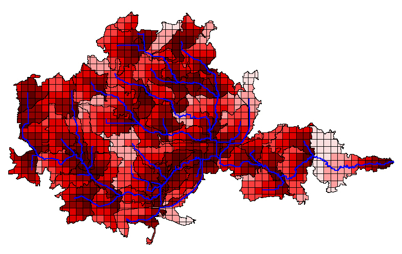
Figure 13: ModClark SHG Cells With Travel Distances
The NEXRAD rainfall at stage III indicated that the radar rainfall has undergone automatic and interactive ground truthing with rain gages. The radar rainfall has been developed in SHG at 1000-meter resolution. The radar rainfall is stored as a series of grids at 5-minute intervals in DSS. The inputs for the precipitation model are shown in Figure 14.
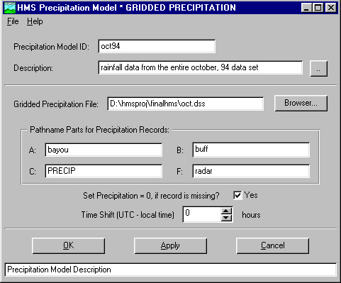
Figure 14: Precipitation Model
The control specifications model identifies a time window for October 16-25, 1994. The computational time interval is set at 5 minutes. The time-related data inputs for the control specifications model are shown in Figure 15.
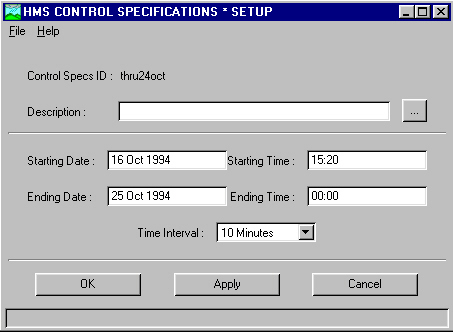
Figure 15: Control Specifications Model
An HMS run consists of a basin, precipitation, and control specifications component as shown in Figure 16. Comparison of HMS computed flow hydrograph with the USGS observed streamflow hydrograph at gage located near West Little York Road on Langham Creek is shown in Figure 17. The HMS computed peak flow compares well with the USGS observed flow; however, the HMS model still needs parameter calibration and model refinement for the reservoirs.
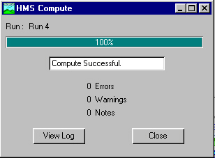
Figure 16: HMS Flow Computations for a Run
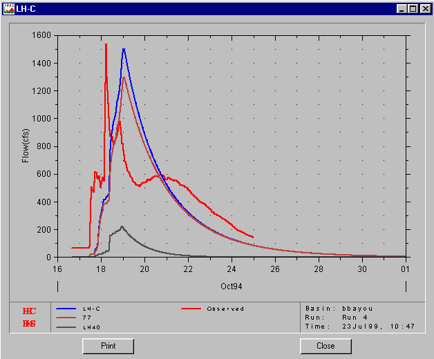
Figure 17: Comparison of Computed and Observed Hydrograph for Langham Creek
Conclusion
In the 1970s, the Hydrologic Engineering Center (HEC) participated in developing some of the earliest Geographical Information System (GIS) applications, such as Hydrologic Parameters (HYPAR) and Spatial Analysis Methodology (SAM), to meet modeling needs in water resources. These early applications were capable of accessing a geographic multi-variable grid cell database and developing unit hydrograph parameters. Since then, HEC occasionally participated in the development of GIS applications to keep abreast with the latest technological advances in hydrology and hydraulics. In the 1990�s, HEC became aware of the phenomenal growth and advancement in the GIS. The capability of obtaining spatial data from the Internet coupled with powerful algorithms in software and hardware made GIS an attractive tool for water resources projects.
This Buffalo Bayou project, funded through the Galveston District of the US Army Corps of Engineers, demonstrates that the development of a quasi-distributed hydrologic model in the Hydrologic Modeling System (HMS) is practical with the aide of GIS software and spatial data. The Galveston District plans to use the HMS model for the Buffalo Bayou watershed, located west of Houston, Texas, as the first step to the long-term needs of the Water Control Data System (WCDS). The WCDS is a streamlined collection of programs and hydrologic, hydraulics, reservoir simulations models for real-time monitoring, active warning, and forecasting of floods. The following sections summarize the accomplishments, obstacles, and recommendations for the project.
The GIS spatial database and the HMS model with ModClark quasi-distributed transformation of grid-based NEXRAD radar rainfall serves as an effective foundation for building the remaining models for the WCDS project as shown in Figure 18. From the GIS standpoint, a finer resolution DEM should be obtained to accurately represent the low-relief terrain and significantly improve the stream and subbasin delineation. The spatial data layer for the hydraulic structures should catalog other drainage structures for the development of a hydraulic model. From the hydrologic standpoint, the Galveston District should review the approach taken in re-using of HEC-1 parameters as demonstrated with the Bear Creek. When concurrence on the approach is reached by Galveston District and HCFCD, Galveston District should continue to recycle HEC-1 parameters, or otherwise develop more refined HMS parameters for the remaining subbasins and streams. Finally, Galveston District should assess the value of Reservoir Simulation System (RSS) for modeling the operations of the Addicks and Barker Reservoir because RSS has been streamlined to be compatible with the WCDS implementation.
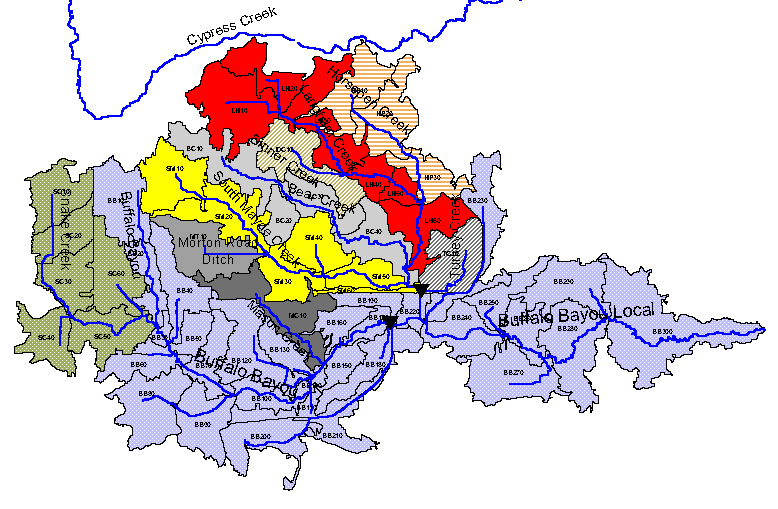
Figure 18: Buffalo Bayou Model Derived in GIS
Author Information
James H. Doan, P.E.
US Army Corps of Engineers
Hydrologic Engineering Center, Davis, CA.
609 Second Street
Davis, CA 95616-4687
Tel. (530) 756-1104
Fax. (530) 756-8250
Email. james.h.doan@usace.army.mil