Breaking Down Jurisdictional Barriers: A Technical Approach to Regional Crime Analysis

Originally, the GIS Staff had intended a third iteration of the pilot project for a large police department. Instead, it was decided to take on a regional project, and so work began on RCAGIS, the Regional Crime Analysis Geographic Information System.

This project, chaired by GIS Staff Chief John De Voe and Phil Canter of the Baltimore County Police Department, takes advantage of a relationship that had already been built among a group of local law enforcement agencies, the Regional Crime Analysis System, or RCAS. The RCAS group formed in 1994 in response to a series of crimes crossing jurisdictional boundaries. Some of the affected organizations decided to share data in hopes of quicker response times in future cross-jurisdictional serial crimes. The RCAS group decided to make use of software developed in-house by the Baltimore County police, the Baltimore Crime Analysis System database (BCAS) and its accompany data entry and query software, BCAP (Baltimore Crime Analysis Program). Meetings were held to decide how best to adapt the existing database and software to best work for the consortium, and server space to hold the software was provided by the Washington Baltimore High Intensity Drug Trafficking Area (HIDTA). The result was the RCAS database and RCAP entry and query software.

At present, data are collected at each participating jurisdiction and uploaded to the database on the HIDTA server as often as desired by the jurisdiction. Each jurisdiction can then download, at their convenience, updates of the master database. Of course, the database’s currency depends on how often the police departments submit data, and the timeliness of the data used for analysis, likewise depends on how recently the jurisdiction has downloaded an update. Ideally, a live system would be instituted in which data are automatically submitted to the master server, and queries of the database are made directly to that server, rather than a local, static copy, but this would require much more of an investment in a telecommunications infrastructure within the consortium.

It was to this framework, an existing consortium with a common database structure already in use, that the Department of Justice was introduced.

At first, it was thought that the existing SCAS package would simply be adapted to the RCAS data structure, with a new front end interface and query wizard interface. SCAS, the Criminal Division GIS Staff’s first project, was ArcView-based, and made use of Esri’s Spatial Analyst extension to generate crime hotspots. Together, these two packages retail for several thousand dollars. Because SCAS was designed to be run by just a few analysts, however, this cost was not seen as terribly prohibitive. With RCAGIS, however, the goal is to put the package in many jurisdictions within a region, and have it available to not just analysts, but street-level officers and management as well. The cost of deploying the application would have quickly grown untenable.

In order to keep costs down, the decision was made to code RCAGIS in Visual Basic 5.0, using MapObjects as its geographic engine. Additionally, CrimeStat, a spatial statistics package developed by Ned Levine and Associates under a grant from the National Institute of Justice, was chosen as a statistical back-end to handle the generation of density surfaces, nearest neighbor analyses, and other such statistics.

MapObjects has a runtime license requirement which would cost roughly $100 per installed machine, and the use of CrimeStat is free within the law enforcement and criminal justice research community. All other components used in the authoring of RCAGIS allow free run-time distribution.

This paper will present an overview of RCAGIS, as well as an in-depth look at some of the technical issues involved in the project and how they were approached.

An RCAGIS session begins at a title screen (Figure 1) which presents the user with three buttons. The first and second of these, the QuickMap and Mapper/Analysis buttons lead the user first through a query wizard and then to a map display window. The third button provides quick access to some of the automated reports which have been created using Crystal Reports 7.0 Professional.

Figure 1:  Title Screen / Main Menu

The wizard (Figure 2) used for query design leads the user through the selection of a jurisdiction, type of geographic area within that jurisdiction (such as police beats or precincts; census tracts; or neighborhoods), time and date range, and crime types. At any time after selecting a jurisdiction, the user may select a "finish" button to complete a map. The specification of jurisdiction and geographic area is done to set various parameters such as shifts (for time-based queries).  Queries generated by RCAGIS are designed to return data for the entire region, rather than just for the area specified. The GIS Staff learned from previous experience in designing crime analysis GIS that users will often go out of their way to avoid looking at incidents outside of their immediate responsibility, so users are automatically presented with data that extends geographically beyond their immediate concerns.

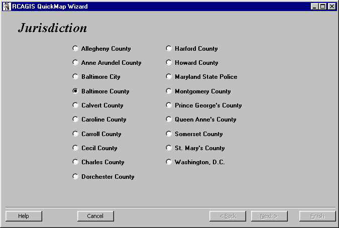Step 1	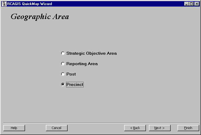Step 2	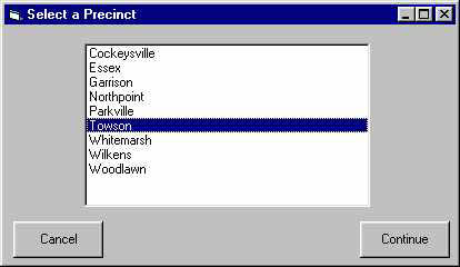Step 2a
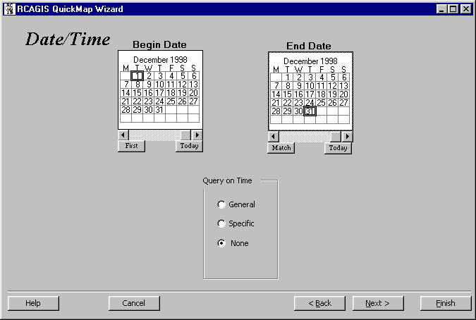Step 3	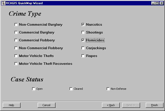Step 4	Step 5

Figure 2:  QuickMap Wizard Steps

In addition to the steps listed above, the wizard also contains screens for selecting additional query attributes such as property stolen, location, and modus operandi. These more detailed queries are available only after selecting the Mapper/Analysis button. The QuickMap was designed to be runnable, start-to-finish, in under one minute.

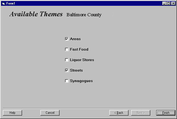
After finishing the last step of the wizard, the user is presented with one more screen, which allows them to specify the sorts of data layers they would like to see on the initial display. Themes can also be turned on and off later from the map display.

The map display has two interfaces, one simple, and one complex. In addition to a large map, both feature a small locator map and legend, as well as simple tools including pan and zoom, map tips, and labeling, crime alert display, printing of map layouts, and access to reporting tools. The complex interface also allows access to spatial statistics, the ability to add and remove themes, edit theme symbology. A toggle is provided so that the user can switch between the simple and complex interfaces. When a user chooses the QuickMap option, they are, by default, presented with the simple interface. When they select the Mapper/Analysis option, they are presented with the complex interface.

Figure 3:  Map Display

The complex interface includes a floating tool window (Figure 4) which gives access to miscellaneous functions related to analysis, both internal to RCAGIS and also requests farmed out to secondary analytical packages such as Ned Levine & Associates' CrimeStat. CrimeStat is a spatial statistics package which is specialized to perform calculations useful in crime analysis.   Some of the functions included are spatial distributions (mean, median, and standard deviation ellipse), spatial autocorrelation (Moran's I, Geary's C), nearest neighbor analysis, hotspot analysis (nearest neighbor hierarchical clustering, k-means clustering) and interpolation (kernel density estimate).

RCAGIS itself does no spatial statistics of internally.  Instead, it launches a CrimeStat session and uses that as an engine to perform analyses on the data currently being examined.  Using Dynamic Data Exchange, a method of passing information between programs in Windows, RCAGIS is able to automatically set parameters for the different functions available in CrimeStat.  When CrimeStat has finished its calculations, it can produce output as a shapefile; the user can then load the produced shapefile into RCAGIS.

A non-statistical analytical operation which is supported by RCAGIS is the ability to draw lines which connect point features in different themes based on a matching key.  This is implemented in a tool which will connect vehicle theft incident locations with the locations at which the vehicle was recovered, and a similar tool which draws connections between incident locations and the home address of the arrestee for that crime.

The tool window also has several tools for the sub-selection of incidents from a query’s return set.  These subsets can be based on user-drawn polygons, selection of points near line features, and so forth.

Auto Recovery Surface

Nearest Neighbor Analysis Linkage Lines

Figure 4:  Analysis Tool Menu, Sample Maps

Reports in RCAGIS are generated by Seagate Crystal Reports 7.0 Professional via ODBC (as described in Appendix B).  There are two different types of reports within RCAGIS; summary and crime alerts. There are four distinct variations of summary reports; crime incident summary, auto thefts, day/time summary, and CrimeStac. The crime incident summary report includes information about the date, time, location, and modus operandi for each crime. The auto theft report shows the make, model, year, stolen address and recovered address of stolen autos. The day/time summary counts the number of crimes that occur for each hour and day of the week. Finally, the CrimeStac counts the number of crimes that occurred for a given for a time period and compares it to previous time periods. CrimeStac is the police management technique used in Baltimore City, and is modeled after the CompStat process popularized by New York City.

The other report that is available is crime alerts. A crime alert is a notice containing information from the incident database, as well as ancillary information that a crime analyst may enter specifically to explain or describe a series of related incidents. For example, if a crime analyst identifies a group of crimes with a similar modus operandi, a crime alert can be created describing the series of events. The crime analyst spatially selects the crime incidents from the map view or key enters the unique crime incident number(s). After the crime analyst has selected the crime incidents a query is made to the crime database that returns pertinent information about the selected crimes such as location, time, target and suspect information. The information appears on a data entry form for the analyst to edit and to enter additional summary information. When the analyst submits the data entry form all of the information that was entered into the data entry form, as well as, the coordinates of the minimum bounding rectangle (MBR) of the selected crimes are stored in a crime alert database and a crime alert notice is generated. The MBR is stored in the crime alerts database, and is used to flag the RCAGIS user whenever a query result overlaps the region encompassed by the crime alert. In addition, existing crime alerts can be edited if new information becomes available regarding the incidents covered in an already created crime alert.

One of the requirements for RCAGIS was the ability to print maps.  The plotting capability was designed to enable RCAGIS users to generate high quality hard copy maps with common features such as text, legends, logos, and scales.

A suite of plotting functions were developed which handle a variety of tasks including low-level functions for tasks such as scale conversions between display and printing devices. Higher level functions include wrapper functions for specific printing commands such as ‘PlotMap’. An essential assumption to the way the RCAGIS printing functions work is that all output is ultimately destined for a printer. Thus all plot commands accept real world page coordinates, in inches, for positioning plot objects on the page. All of the plot functions are written to be hardware-independent, and take an .hdc (Hardware Device Context) as an argument. The output device can be either a form, or the current Windows default printer. If the output is directed to a form, then the form is scaled to exactly match the aspect ratio of the current printer page size, and all plot function coordinates are scaled to match the relative size of the form. This enables the display form to be essentially WYSIWYG (What You See Is What You Get).  This methodology simplifies the inclusion of a print preview function.

Figure 5:  Printing

As implemented in RCAGIS, all printing commands are called from plot commands in a text ‘layout’ file. The layout files are, by default, stored in the /layouts subdirectory of the RCAGIS home directory. For user convenience, the currently selected layout file can be edited in Microsoft Notepad by clicking the ‘Edit’ button in the ‘Map Options’ dialog box. Each plot command has several arguments, the minimum requirement being location coordinates for the location on the printed page. The layout file permits police departments to create map ‘templates’ which provide a consistent look and feel for the maps. The available plot commands, the names of which fairly well describe their function are: plotbitmap, plotbox, plotdate, plotlegend, plotlocatormap, plotmap, plotnortharrow, plotpageborder, plottextscale, and plotreferencegrid.  A sample layout file can be found in Appendix C.

While RCAS was able to provide a unified data structure in use by its members, this addressed only the incident, suspect, and stolen vehicle recovery data. Because each jurisdiction maintains its own geographic base files, with different levels of detail, attributes, and even projections, one of the needs of the RCAGIS project was to provide a way to organize and view disparate geographic files in a way that would provide context for the incident data. Rather than worry about whether or not boundaries were perfectly aligned, or streets crossing jurisdictional lines would be perfectly connected, the design team wanted to make sure that the crime data was at the forefront, and that the user be able to see data on both sides of a border.

Additionally, a large degree of flexibility was requested by the members of RCAS. For instance, although a list of required queryable crime types was provided, some jurisdictions felt that they should be able to include other options. Other jurisdictions were interested in being able to map data from sources other than the standard RCAS database.

A number of different techniques were used in RCAGIS to accommodate the goals of the project. To increase the flexibility of the software for administrators, large portions of RCAGIS’ behavior and interface are modified at run time, allowing multiple configurations of the package based on a given user’s or group of users’ needs. This is particularly noticeable in the wizard, in which the contents of every screen can change based on values in a local configuration database.  To try to cut down on the confusion caused by having disparate source data, particularly for multiple files representing, in effect, a single type of feature, an architecture that allowed the integration of multiple shapefiles into what appear to the user as single themes was created. An integrated method of handling with projections within and across jurisdictions was designed.  Some of the custom objects and architectures used to make all of this work will be examined below, along with descriptions of the additional support applications which were written to provide administrators with the ability to make these features fit their needs.

MapObjects loads shapefiles as individual layers within a map display object. Ordinarily, each of these layers would be displayed in a legend. However, since each jurisdiction brings different shapefiles, often for the same or similar type of geographic feature, it was felt that this would not only clutter the legend, but also be confusing to the user in that two shapefiles representing the same type of data might be displayed at different levels on the map – streets might plot over land use for one jurisdiction, but under land use for another.

To solve this problem, the idea of a theme was created. A theme, in effect, is a collection of shapefiles with which the user can interact as if it were a single map layer. Users can add and remove, turn on and off, and modify the display order of entire themes – automatically acting on each shapefile-based layer within that theme – seamlessly. Furthermore, administrators may define symbols for the individual features of shapefiles such that they will look like other shapefiles displayed within the same theme.   The Symbolizer application, discussed below, is the primary means provided to administrators for editing these symbols.

The first step of implementing themes was to create a way to load and save legends for individual shapefiles. These legends are stored as plain text in files with an .rvl extension, typically using the same prefix as the shapefile they are to accompany. Because it was desirable to be able to symbolize a shapefile differently at different scales (for instance, providing less detail on a road layer at small scales), the legend files were designed so that they could store multiple legends, each with a specified minimum and maximum display scale.

MapObjects uses renderer objects to symbolize map layers. Each renderer has a set of attributes, some of which apply to all renderers (e.g. color) while others apply only to particular type of renderer (e.g. DotValue). Legend files may store any of the types of renderers included in MapObjects 1.2, as well as the LabelPlacer object, and may store different types of renderers for use at different scales. Legend files can also store alternate captions to use for display in an ArcExplorer-styled legend. For instance, if an attribute in the database reads "W", one might wish to assign the word "Water" for a more meaningful display. Finally, legend files can also store an arbitrary string which allows specification of a theme type; this is what allows shapefiles to be grouped into themes as described above.

In order to actually handle the multiple renderers that might be used with a single layer in a map, the ScaleRenderer object was created. The ScaleRenderer  is basically a collection of renderers, along with details about the scales at which each is to be used, and containing information about the layer being symbolized – to which jurisdiction, if any, it belongs; the type of layer (streets, schools, land use, etc.), and whether or not that jurisdiction is currently visible on the map display.

Another object, the ScaleRenderers collection, was also written to handle the overhead of keeping track of the multiple ScaleRenderer objects that would be needed for a map. The ScaleRenderers collection holds a ScaleRenderer for each layer loaded into a map. For any given layer, it can return the correct renderer to use for the current display scale. It can also return subsets, such as a reference to all of the loaded layers of a given type. In order to be able to identify which ScaleRenderer in the collection is to be used for a given layer in a map, the layer’s tag is specified as the full path and filename of the shapefile. This same string is then used as the key for that layer’s ScaleRenderer within the ScaleRenderers Collection.

To simplify use of the ScaleRenderer and its collection, an automated method of loading a shapefile with its attendant legend file into a map layer was written. The programmer simply passes the ScaleRenderers collection, along with a few other necessary things such as the map layer (to ensure its tag is correct) and the shapefile’s path and filename, and a new ScaleRenderer is added to the collection.

Using the ScaleRenderers collection is fairly simple. In a map’s BeforeLayerDraw event, one cycles through the layers, using the layer tag as a means to get to the ScaleRenderer containing symbology information for the layer and thereby retrieve the correct renderer for the current scale.

Because one of the goals of the theme architecture was to cut down on clutter in a legend display, a fairly extensive rewrite was performed on Esri’s ArcExplorer legend ActiveX control, the source code to which was included in the MapObjects 2 distribution. The ArcExplorer legend is a fairly simple control with many useful features. When associated with a map control, it will display a list of the layers loaded into that map. Map Layers include a small set of symbols representing the settings of the renderer or symbol used to draw the layer. An optional checkbox gives the user control over whether a layer is visible. Users may reorder the layers of a map by dragging and dropping the items listed within the legend. A single layer may be specified as "active" by clicking on it; the legend can then be queried for the active layer so that operations can be carried out on the specified layer.

The new version, legendSR, is backwardly compatible with the old legend, and now contains a property for storing a reference to a ScaleRenderers collection. If this property has been set, the legend will ensure that its display reflects what is currently displayed in the map window based on scale. Further, to help in situations in which two jurisdictions might use different shapefiles with varying legends for the same theme, the legend will display the symbology for the shapefile which is currently in the center of the map display.

If a ScaleRenderer contains alternate captions for the values a renderer will display, the legendSR will use the alternate captions. Theme names are used to identify the item in the legend, rather than the name of the individual layer. And of course, the legendSR ensures that when themes in the legend are dragged up or down, all of the layers with that type will move up or down in the map draw order so that they remain together.

Further support of the Themes architecture was written into a new version of Esri’s MapTip class, distributed as part of the MOView sample in MapObjects 1.2. MapTips allow the user to specify an attribute field of interest; hovering over a feature on the map will pop up a small label showing the value of the attribute field for that record. The new version of the MapTip object is capable of displaying MapTips for multiple shapefiles which have been grouped into a theme. The only limitation to this is that the user may only specify one attribute name on which to search. However, if the shapefiles share field names, such as "Name," this will not cause problems.

One of the requirements for RCAGIS was that the software be able to display image layers – or more specifically, to be able to take advantage of the aerial digital orthophotos available to some members of the consortium.

MapObjects image layers can not be projected. In order to display shapefiles on top of a georeferenced image, one needs to specify the coordinate system of the map display as well as the coordinate system of the shapefile, if it differs.

Ideally, all shapefiles used in RCAGIS could be converted to a common projection, which would obviate the need to project shapefiles for display. However, unless any image layers, such as aerial photos, that participatory jurisdictions wished to use were all in the same projection, it would still be necessary to specify input and output projections for the displayed shapefiles and map control, respectively.

One of the new features of MapObjects 2 is the ability to handle multiple projected and unprojected coordinate systems. By breaking it down such that a map object has an display projection and shapefiles have, in effect, input projections, it becomes possible to display shapefiles with two different projections in a third projection! RCAGIS takes advantage of these projection capabilities, allowing jurisdictions to maintain their data in a locally prescribed projection, yet still view their data alongside that from other jurisdictions or sources, while allowing these data to be viewed over an image layer with an unchangeable projection.

In order to handle the projections that would be necessary within RCAGIS, an object called the ProjectionDictionary was created. Ordinarily, a projection file, with the extension .prj, would be stored with each shapefile. By assuming that projection files, if they exist, should be loaded and assigned to a layer, geographic data would need to be, in effect, unprojected and reprojected even if the input and output coordinate systems are identical. Instead, RCAGIS stores projections in its internal configuration database, and specifies the projection to be used for each given shapefile. The primary advantage to this is that projections are only assigned to input layers if their projection is different from the output projection. In other words, if a shapefile has been stored as UTM coordinates and the map will be projected to UTM, the layer’s CoordinateSystem property is set to nothing. This yields a noticeable improvement in map display speed.

Rather than force RCAGIS administrators to define a projection for every shapefile utilized within a jurisdiction, defaults can be assigned to jurisdictions. For instance, if the bulk of the data used by a jurisdiction is in Maryland State Plane, than that can be assigned as the default projection for the jurisdiction and all shapefiles associated with that jurisdiction will be assumed to be stored in that coordinate system unless otherwise specified. Individual projections may be specified for themes and geographic areas.

The projections themselves are stored within the configuration database, rather than as individual .prj files. The ProjectionDictionary object automates the tasks of importing projection files into the database and retrieving them from the database as coordinate system objects. Internally, the database stores the contents of projection files in a memo field. When a request is made to an instance of a ProjectionDictionary to retrieve a projection which has not yet been stored as a coordinate system object within the instance, the dictionary will write out a temporary projection file containing the text describing the protection; use MapObjects methods to open that file as a coordinate system, and then remove the scratch file. Subsequent requests for that same projection will be able to use a reference to the now-loaded object.

In many ways, the ProjectionDictionary simply acts as an interface to data stored within the configuration database. It provides a single object that allows storing and retrieving projections, conversion of Arc/Info projections to MapObjects projections, and exportation of shapefiles into new projections.

While RCAS provided a unified data structure to which all members of the consortium had agreed to conform, the reality is that they also wanted the flexibility to specify other data sources, other shapefiles, other attributes.

The RCAGIS wizard interface sets a number of parameters for the map display, such as the area to which the map extent will be set. But its main purpose is to generate the SQL queries necessary to extract incident, arrestee, and vehicle recovery data from the incident database. These query strings are then passed to a module which actually performs the query and creates shapefiles out of the geocoded data returned from the database. The actual data transfer occurs through ODBC, the Open Data Base Connectivity standard, which allows software to communicate with databases through a standard application programming interface.

The shapefiles which RCAGIS exports contain a very limited number of attributes, typically just a unique key, crime classification, and x and y coordinates. Additional attributes contained in the database can then be linked to the shapefile via MapObject’s AddRelate method. The output shapefile field names are standardized, but the names of the fields which provide the data from the source database are editable. The mechanism to specify a series of fields or formatted fields to join to the exported shapefile uses a stored query, thus allowing administrator to specify which additional attributes will be visible within RCAGIS, and how they will be displayed.

There are several advantages to this architecture. RCAGIS is not tied to a single database vendor, because it uses ODBC to connect to the database. It also becomes more flexible by not stipulating that the source database must contain certain tables with specifically named fields. And finally, after benchmarking tests were performed in which the speed of exporting a large number of attributes to the output shapefile was compared to outputting just a few fields and then using an AddRelate to bring in other data, it was found that the AddRelate method was approximately twice as fast.

Sitting behind RCAGIS are two databases. One, of course, is the incident database from which RCAGIS creates its maps. The other is a database which defines the way RCAGIS will behave. From the shifts that are associated with a jurisdiction, to the projections available for use in displaying data, to the Structured Query Language (SQL) code which defines the way the incident database is queried. Administered with a stand-alone tool, configuration database allows RCAGIS to be customized.

When RCAGIS runs, it uses information contained in the configuration database to build its wizard menus on the fly. Multiple configurations may be created, with a single one chosen on RCAGIS-startup by an advanced user.

The configuration database contains jurisdiction-specific information, including the default projection, the shapefiles which fit the theme types available, shift definitions, and the geographic areas available.

Geographic areas have their own set of attributes. Because police geographies may change with the time of day (e.g. post boundaries may be different between a day shift and an evening shift), geographic areas can be based on either one or multiple shapefiles, and in addition to the shapefile(s) which defines the area, also include information such as the fields used to define the names or other identifiers of the areas, and whether the default projection or an alternate should be used for display.

Finally, for each jurisdiction, the administrator may define which theme types are available and specify the shapefile to use. As with the geographic areas, the individual shapefiles in a theme may use either the default projection for the jurisdiction or an alternate.

There are also a number of global items which may be altered. The administrator may also configure the crime types that will be available within the wizard. New crime types are given a name and then assigned three SQL queries, one each for open, closed, and non-defense cases.

The field assignments used to generate result, recovery, and arrestee shapefiles may be specified, along with the names of stored queries to use in the AddRelate of attributes to exported shapefiles. One can also specify the default output coordinate system of the RCAGIS map display and a default input coordinate system which will be applied in cases where no projection information (at the jurisdiction level, or otherwise) exists. By default, RCAGIS assumes that such shapefiles are for a NAD 83 geographic coordinate system.

To aid in the distribution of geographic data between members of the regional consortium, a method of importing and exporting configuration and geographic data was developed. The export files generated are actually zip archives which contain everything from a partial configuration database including all necessary information about shifts, identification numbers, geographic areas, and themes, to all of the shapefiles and legends which are available for that jurisdiction. Obviously, these export files can grow quite large, particularly if such things as street network files are included.

When a jurisdiction export file is created, the software finds all of the records in different tables in the configuration database which pertain to that jurisdiction. These records are written into matching tables in a new database, created in scratch space. The Administrator program then starts a subprocess of Info-Zip’s freeware zip.exe program and creates an archive containing the temporary database as well as all of the shapefiles (with legends) referenced for that jurisdiction.

When importing a jurisdiction into a configuration database, the shapefiles and temporary database are extracted. The software then adds the records for such features as geographic areas, shifts, and themes back into the target configuration database, updating key values as necessary to maintain referential integrity between tables.

Figure 6:  Administrator

The RCAGIS Symbolizer is a stand-alone tool which allows the user to create, save, and load RCAGIS legend files (.rvl). The Symbolizer can be pointed to an RCAGIS configuration database and thus will support projections and theme types as defined within RCAGIS.

The main work of the Symbolizer is carried out by a legend editor menu. Though similar to the legend editors included in the MapObjects example MOView and Esri’s ArcExplorer, this RCAGIS legend editor allows the user to create and define multiple legends for a single file, based on the range of display scales in which each legend is to be used. Further, each legend or group of legends can be assigned the type attribute which is used to create multi-layer themes. Legends for one shapefile may be loaded and applied to another shapefile, and while legends are by default saved alongside the shapefile which they represent, alternate names and locations may be specified.

Figure 6:  Symbolizer Layer Properties

Configuration Selector:

With all the flexibility that was designed into RCAGIS, there was a desire to not immediately lock it up again to the user.  Rather than allowing administrators to specify just one incident database or configuration database, or even at a lower level such as the default layout files available for printing, all of the applications in the RCAGIS suite have the option of starting with a dialog box which allows the user to specify a set of options to use.  These include pointers to the incident database, ODBC Data Source Names, spatial data directories, and so forth.

In Symbolizer and RCAGIS itself, the Configuration Selector can be launched by running the program with the parameter "config."  The Administrator tool automatically starts with the Configuration Selector.

When new configurations are created, the user moves through a series of tabs and sets various path, spatial data, and database connectivity attributes.  After these attributes have been set, they are then saved in the system's registry, along with a specification of which configuration should be used by default, should the user start the application without the config parameter.   Configurations may also be saved and loaded.  RCAGIS is distributed with a default configuration file to simplify the installation of the software.

Configurations

Database Options

Paths

Figure 8:  Configuration Selector

The decision to use Visual Basic and MapObjects to develop RCAGIS had the effect of both drastically lowering the cost to deploy the application while dramatically improving its flexibility.  This flexibility does not come without a cost; the nature of MapObjects is such that any and all functions required by an application must be programmed.  While the use of object-based technology and code reuse can help simplify and speed the task, it must still be remembered that the task itself becomes much larger when building a system largely from scratch (even with the use of library of geographic tools such as MapObjects), rather than layering it on top of an existing application such as ArcView, the platform on which the GIS Staff based its SCAS application.  However, for the flexibility that this approach afforded --including the sheer number of tasks that would have been impossible in a structured environment such as ArcView -- there is a definite pay-off.

The initial development of RCAGIS is currently nearing completion, and testing is being carried out by members of the RCAS consortium.  Source code to the entire package will eventually be disseminated through the Department of Justice web site at http://www.usdoj.gov/criminal/gis

Appendix A:  Object Models

The following are draft class diagrams for some of the objects discussed in this paper.

The RCAGIS version of Esri's MapTip class has integrated support for themes, allowing the user to identify features which appear to be in the same map layer, but are drawn from multiple shapefiles.

The ProjectionDictionary is a collection of MapObjects coordinate systems which can be assigned to MapLayers or Maps.  It also acts as in interface to the projection information stored in an RCAGIS configuration database.

The ScaleRenderer object maintains multiple renderers along with parameters specifying the scales at which each will be used.  The ScaleRenderer can also maintain a type property which allows multiple layers to be treated as a single theme.

The ScaleRenderers collection provides a convenient way of storing and manipulating ScaleRenderer objects.  The collection is keyed by the tag of the layer represented by a given ScaleRenderer, so that the software can quickly retrieve the correct renderer for a given layer at a given scale.

Seagate’s Crystal Reports 7 was used to create all of the reports within RCAGIS. Each report template is designed to generate a report via Open Database Connectivity (ODBC). ODBC is a standard developed by Microsoft that allows applications to communicate to a variety of databases through a single process. In order to use ODBC the ODBC source name has to be configured. The ODBC source name allows applications to communicate with a specific database. Once ODBC has been installed and the ODBC source name has been configured RCAGIS can generate reports.

ODBC AND CRYSTAL REPORTS

The report generation process via ODBC goes through five layers; the Seagate Crystal Reports layer, ODBC translation layer, ODBC layer, Database Management Systems (DBMS) translation layer and database layer. The Seagate Crystal Reports layer creates the Structured Query Language (SQL) statement to request the appropriate data. SQL is a programming language for organizing, managing, and retrieving data stored in a database. The SQL statement can be generated by Crystal or passed to the Crystal object. The ODBC translation layer is the driver that passes the SQL statement and data to and from ODBC. The ODBC layer is the gateway that allows several databases to communicate to other applications. ODBC determines which ODBC source name will process the request. The DBMS translation layer (ODBC DSN (data source name)) specifies the location of the database to query. Finally, there is the database layer. This is the source of the data that will used to generate a report.

ADVANTAGES AND DISADVANTAGES OF ODBC

There are four advantages of using ODBC to generate reports. First, ODBC drivers exist for all major databases. Second, it is flexible because if you change databases few modifications are required to the SQL string. As long as the database tables and field names are the same the only modifications required are reconfiguring the ODBC source name and editing the SQL statement, if necessary. Third, you have access to all the tables and data through one interface. Finally, most of the work is done on the server with the SQL pass-through technology. This means there will be less network traffic and frees up more memory on the local computer.

Some of the disadvantages of using ODBC are that it may take more time to generate a report than other directly accessed data sources. With ODBC there are so many layers it must go through it has a chance to fail at any one of these layers. Also, the data source name has to be configured before any reports can be generated. Finally, SQL syntax can differ from database to database. A SQL statement sent to a DSN may work for one database but not for another.

Layout files are plain text stored in files with an extension of .lyt which can be edited with any text editor, including the Windows NotePad program.  Lines beginning with an apostrophe are comments.