Figure 1: Raster-based functions for terrain analysis for hydrologic
purposes.
19th Annual Esri International
User Conference
July 26-30, 1999
San Diego, California
GIS Tools for HMS Modeling Support
Francisco
Olivera and David
R. Maidment
Center for Research in Water Resources
University of Texas at Austin
Austin, Texas
Abstract
CRWR-PrePro is a system of ArcView scripts and associated controls, developed to extract topographic, topologic and hydrologic information from digital spatial data of a hydrologic system, and to prepare ASCII files for the basin and precipitation components of HEC-HMS. These files, when opened by HEC-HMS, automatically create: (1) a topologically correct schematic network of sub-basins and reaches attributed with hydrologic parameters, and (2) a protocol to relate gage to sub-basin precipitation time series. Starting from the DEM, CRWR-PrePro delineates the sub-basins and the reach network, calculates parameters for each hydrologic element, determines their interconnectivity, and prepares an input file for HEC-HMS that includes the computed hydrologic parameters. CRWR-PrePro also generates an input file for the precipitation component of HEC-HMS. Two methods to interpolate precipitation records are supported: one to calculate average precipitation at the sub-basins based on Thiessen polygons, and another to calculate the routing parameters of precipitation cells for hydrograph determination. Using CRWR-PrePro, the determination of the spatial parameters for HEC-HMS is a simple and automatic process that accelerates the setting up of a hydrologic model and leads to reproducible results.
1. Introduction
2. Previous Work
3. Methodology
4. Conclusions
Acknowledgements
References
Author Information
Rainfall runoff modeling and flood discharge estimation have always been important tasks in hydrologic sciences and engineering. Flood flow estimation, in particular, has been given special attention because of the impact that accurate forecasts have in the management of flood-related emergency programs. Probably more than other concerns in hydrology, estimation of flood discharges is oriented towards saving human lives and protecting people's property.
The Hydrologic Modeling System (HMS), developed by the Hydrologic Engineering Center (HEC) of the United States Army Corps of Engineers (USACE), is a software package used to model rainfall runoff processes in a watershed or region, and is a further development of the well-known HEC program HEC-1. For rainfall runoff modeling, HMS requires three input components:
The first two components, basin and precipitation, depend strongly on spatial factors, so geographic information systems constitute a powerful tool to generate this type of input data.
CRWR-PrePro is a system of ArcView scripts and associated controls, developed to extract topographic, topologic and hydrologic information from digital spatial data of a hydrologic system, and to prepare ASCII files for the basin and precipitation components of HEC-HMS. These files, when opened by HEC-HMS, automatically create: (1) a topologically correct schematic network of sub-basins and reaches attributed with hydrologic parameters, and (2) a protocol to relate gage and sub-basin precipitation time series. CRWR-PrePro has been developed at the Center for Research in Water Resources (CRWR) of the University of Texas at Austin, and supersedes the former CRWR package HEC-PrePro. Additional capabilities of CRWR-PrePro with respect to HEC-PrePro include the relaxation of the one-to-one sub-basin/reach relation which was enforced in the previous version, sub-system extraction by selecting the downstream sub-basin polygon, and preparation of an input file for the precipitation component, among others.
HEC-HMS is a very flexible program that allows the user to choose among different loss rate, sub-basin routing, and baseflow models for the sub-basins, as well as different routing methods for the reaches. However, because some of these models and methods depend on hydrologic parameters that cannot be extracted from readily available spatial data, CRWR-PrePro does not estimate parameters for all of the methods supported by HEC-HMS. At the moment, CRWR-PrePro calculates or imports parameters for:
Using CRWR-PrePro, the determination of the spatial parameters for HEC-HMS is a simple and automatic process that accelerates the setting up of a hydrologic model for HEC-HMS and leads to reproducible results.
The suitability of raster-based GIS for modeling gravity driven flow has been previously addressed in the literature (Olivera and Maidment 1998a, Maidment 1992). Consequently, raster-based GIS algorithms for hydrologic analysis have been developed (Jensen and Domingue 1988, Jensen 1991) and included in commercially available GIS software. Functions to delineate reaches and sub-basins, that use Jensen and Domingue's algorithms, are available in ArcView 3.0a Spatial Analyst 1.1 through Avenue requests and also through the Hydrologic Modeling ArcView extension distributed by Esri with the Spatial Analyst. Likewise, digital elevation models (DEM's) have been developed for different parts of the world at different resolutions (USGS a, USGS b, USGS c), and further developments of these data have been aimed towards improving its spatial resolution. Other spatial data sets such as land use and soil type have also been developed for different parts of the world.
CRWR-PrePro is the synthesis of ArcView applications developed over the last years at the Esri and CRWR. The Watershed Delineator ArcView extension (Djokic et al. 1997, Esri 1997), developed by the Applications Programming group at Esri for the Texas Natural Resources Conservation Commission (TNRCC), can be used to delineate watersheds to a point, line segment, or polygon, selected interactively by the user from the map. The Flood Flow Calculator ArcView extension (Olivera et al. 1997, Olivera and Maidment 1998b), developed at the CRWR for the Texas Department of Transportation (TxDOT), can be used to estimate flood peak flows according to the regional regression equations developed by Asquith and Slade (1997) for Texas. All hydrologic parameters required by these equations, such as drainage area, watershed shape factor and slope of the longest flow path, are extracted automatically from the spatial data. HECPREPRO (Hellweger and Maidment 1999), developed at the CRWR for the HEC, can be used to establish the topology of the hydrologic elements, and write an input ASCII file readable by HEC-HMS with all this information. CRWR-PrePro combines the terrain analysis capabilities of the Watershed Delineator with the hydrologic parameter calculation capabilities of the Flood Flow Calculator and the topologic analysis capabilities of HECPREPRO, to conform a hydrologic modeling tool that prepares -- from ready available digital spatial data -- the input file for the HEC-HMS basin component. CRWR-PrePro uses code originally developed for the Watershed Delineator, Flood Flow Calculator and HECPREPRO, although modifications have been made to meet the specific needs of this system.
Additionally, precipitation interpolation methods, developed at CRWR and HEC, have been included in CRWR-PrePro for determining the HEC-HMS precipitation input component. A Thiessen-polygon-based method (Dugger 1997), developed at the CRWR, can be used to estimate sub-basin precipitation as a weighted average of gage precipitation. GridParm (HEC 1996), originally developed at HEC in Arc Macro Language (AML) and rewritten at CRWR as an Avenue script, can be used to determine parameters of precipitation cells for use with the ModClark sub-basin routing method of HEC-HMS. ModClark, a variation of the original Clark unit hydrograph model, has been developed for HEC-HMS as a sub-basin routing option suitable to support NEXRAD precipitation data.
CRWR-PrePro generates data for the basin and precipitation input components of HEC-HMS.
The process of generating input data for the basin component has been divided into six conceptual modules: (1) raster-based terrain analysis; (2) raster-based sub-basin and reach network delineation; (3) vectorization of sub-basins and reach segments; (4) computation of hydrologic parameters of sub-basins and reaches; (5) extraction of hydrologic sub-system (if necessary); (6) topologic analysis and preparation of the HEC-HMS basin file.
Raster-Based Terrain Analysis
Raster-based terrain analysis for hydrologic purposes uses Jensen and Domingue's (1988) algorithms. By running the flowdirection Avenue request, a single downstream cell -- out of its eight neighbor cells -- is defined for each terrain cell. This downstream cell is selected so that the descent slope from the cell is the steepest. Therefore, a unique path from each cell to the basin outlet is determined. This process produces a reach-network, with the shape of a spanning tree, that represents the paths of the watershed flow system. However, because a flow direction cannot be determined for cells that are lower than their surrounding neighbor cells, a process of filling the spurious terrain pits is necessary before determining the flow directions (Esri 1992). Once the terrain depressions have been filled and the flow directions are known, the drainage area -- in units of cells -- is calculated with the flowaccumulation Avenue request. The flow accumulation grid stores the number of cells located upstream of each cell (the cell itself is not counted) and, if multiplied by the cell area, equals the drainage area. Figure 1 shows an example of how the flowdirection and flowaccumulation requests work when applied to a DEM.
Figure 1: Raster-based functions for terrain analysis for hydrologic
purposes.
Raster-Based Sub-Basin and Reach Network Delineation
The DEM cells that form the reaches are defined as the union of two sets of grid cells. The first set consists of all cells whose flow accumulation is greater than a user-defined threshold value. This set identifies the reaches with the largest drainage area, but not necessarily with the largest flow because flow depends on other variables that are not related exclusively to topography. The second set is defined interactively by the user by clicking on a certain point on the map, which results in an automatic selection of all downstream cells. This capability allows the user to select a particular reach, which might have a small drainage area (low flow accumulation), without having to lower the threshold value for the entire system and defining unnecessarily a denser reach network. After the reach cells have been defined, a unique identification number or grid code is assigned to each reach segment. Figure 2 shows threshold-based and user-defined reaches, as well as their corresponding reach segments.
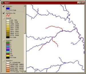
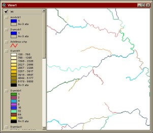
Figure 2: Reach network delineation. In the left-hand-side figure, blue
cells correspond to drainage areas greater than 3000 grid cells, whereas
red cells are defined interactively. In the right-hand-side figure, each
reach segment has been identified with a different grid code and displayed
with a different color.
Sub-basin outlets are also defined as the union of two sets of grid cells. The first set, based on the reach network, consists of all cells located just upstream of the junctions. Consequently, at a junction, two outlet cells are identified, one for each of the upstream branches. The system outlet is also identified as a sub-basin outlet. Since these outlets are the most downstream cells of the reach segments, their identification number or grid code is the same as their corresponding reach segment. The second set is defined interactively by the user by clicking on any cell of the reach network, such as those associated with flow gages, reservoirs or other water control points. The identification number or grid code of each new interactively-defined outlet is obtained by adding one to the highest grid code value available. Reach segments containing interactively-defined outlets are subdivided at the clicked cells, so that the new segments -- upstream of the new outlets -- are assigned the same grid code as their corresponding new outlet. Outlets associated with reservoirs can be identified so that HEC-HMS recognizes them as both, reservoirs and sub-basin outlets. Figure 3 shows threshold-based and user-defined outlets, as well as the corresponding reach segments.
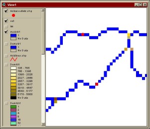
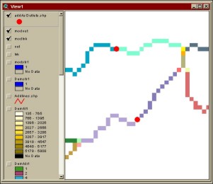
Figure 3: User-defined sub-basin outlets. In the left-hand-side figure,
blue cells represent the stream network in raster format, color cells the
sub-basin outlets located just upstream of the junctions and red dots interactively-defined
outlets. In the right-hand-side figure, each stream segment is displayed
in a different color, and segments containing red dots have been subdivided
into two or more segments.
The watershed Avenue request is then used to delineate the areas draining to each sub-basin outlet. Sub-basins are assigned the same identification number, or grid code, as their corresponding outlet and reach segment. Figure 4 shows the delineated sub-basins and reach network in raster format.
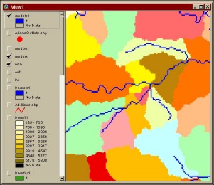
Figure 4: Delineated sub-basins and reach network in raster format.
At this point, a one-to-one relation between reach segments and sub-basins is maintained because a unique sub-basin outlet has been identified for each reach segment. Due to this one-to-one relation, sub-basin and reach segment grid codes are equal.
Vectorization of Sub-Basins and Reach Segments
Because HEC-HMS applies lumped models within each hydrologic element, hydrologic parameters have to be calculated for the sub-basins and reach segments, and not for the individual grid cells. After the reach segments and their corresponding drainage areas have been delineated in the raster domain, a vectorization process is performed using raster-to-vector conversion functions. This process consists of creating a polyline feature data set of reaches, and a polygon feature data set of sub-basins. When doing so, the grid code values are transferred to the attribute tables of the feature data sets, thus preserving a way to directly link sub-basins and reaches. Further vector processing, i.e., merging of dangling polygons, might be necessary to ensure that each sub-basin is represented by a single polygon, and that the one-to-one reach/sub-basin relation established in the raster domain is preserved in the vector domain (Olivera et al. 1998a). Figure 5 shows the delineated sub-basins and reach network after vectorization.
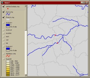
Figure 5: Delineated sub-basin polygons and reach network polylines
after vectorization.
The one-to-one reach/sub-basin relation, though, can be relaxed by merging adjacent sub-basin polygons, so that a sub-basin contains more than one reach. In such a case, a new field is necessary in the attribute table of the reaches to account for the grid code of the sub-basin in which the reach is located after merging polygons. For merging two sub-basins, the polygons have to share the same outlet or drain one towards the other. Figure 6 shows the merging of two sub-basins that share the same outlet, as well as the attribute tables of the sub-basin and reach network data sets before and after the merging.
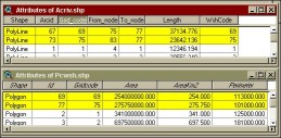
Before merging
After merging
Figure 6: Sub-basin polygons and attribute tables before and after merging polygons. In this case, the two merged polygons share a common outlet.
CRWR-PrePro also has the capability of identifying, for each sub-basin polygon, all the sub-basin polygons located upstream of it, so that they can be easily retrieved when delineating a watershed from a point.
Computation of Hydrologic Parameters of Sub-Basins and Reaches
The sub-basin parameters calculated by CRWR-PrePro are area, lag-time and average curve number. Other parameters needed for estimating the lag-time, such as length and slope of the longest flow path, are also calculated and stored in the sub-basin attribute table. Depending on the algorithm used to calculate the lag-time, it might depend entirely on spatial data, i.e., DEM, land use and soils, or it might require additional externally supplied input. Depending on the method selected, the average curve number can be used to calculate the sub-basin lag-time and the sub-basin loss rate. Figure 7 shows the attribute table of the sub-basins data set with the calculated hydrologic parameters appended.
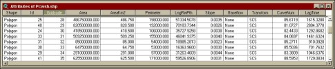
Figure 7: Sub-basin attribute table showing the calculated and appended
fields: area in Km2 (AreaKm2), length of longest flow-path (LngFlwPth),
slope of longest flow-path (Slope), baseflow (Baseflow), sub-basin routing
method (Transform), average curve number (CurveNum) and sub-basin lag time
(LagTime).
The sub-basin area is calculated automatically in the process of vectorizing the sub-basin polygons.
The sub-basin lag-time is calculated with either of the following formulas
 ( 1 )
( 1 )
 ( 2 )
( 2 )
where tp (minutes) is the sub-basin lag-time measured from the centroid of the hyetograph to the peak time of the hydrograph, Lw (feet) is the length of the longest flow-path, S (%) is the slope of the longest flow-path, CN is the average curve number in the sub-basin, Dt (min) is the analysis time-step, and vw (m/s) is a representative velocity of the longest flow-path. In equation (1), the first term in the parenthesis corresponds to the lag-time according to the SCS (1972), whereas the second term is a minimum lag-time value required by HEC-HMS (HEC 1990). In equation (2), the first term corresponds to the lag-time defined as the 60% of the sub-basin time of concentration, and again the second term is a minimum lag-time value required by HEC-HMS. Olivera et al. (1988a) present in detail the methodology to calculate Lw and S from DEM data. On the other hand, values of vw cannot be estimated from spatial data and have to be supplied by the user.
CN is calculated as the average of the curve number values within the sub-basin polygon. A curve number grid is calculated using land use data described by Anderson land use codes, percentage of hydrologic soil group (A, B, C and D) according to STATSGO soils data, and a look-up table that relates land use and soil group with curve numbers (Smith 1995).
Loss rate in the sub-basins can be calculated with either of the following methods: the SCS curve number method for which the average curve number is calculated, or the initial plus constant loss rate method for which the initial and constant rate values have to be supplied by the user. It is likely that in a near future it will be possible to establish a relation between terrain properties and loss rate parameters.
The reach parameters determined by CRWR-PrePro are the length, the routing method (either Muskingum or pure lag), the Muskingum K and the number of sub-reaches into which the reach is subdivided in case Muskingum is used for routing, and the flow time in case pure lag is used for routing. Other reach parameters like the flow velocity and the Muskingum X cannot be computed from spatial data and must be calculated externally and supplied as input. Figure 8 shows the attribute table of the reach network data set with the calculated hydrologic parameters appended.
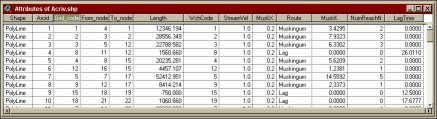
Figure 8: Reach attribute table showing the calculated and appended
fields: reach velocity (StreamVel), Muskingum X (MuskX), reach routing
method (Route), reach flow time in hours or Muskingum K (MuskK), number
of sub-reaches (NumReachN), reach flow time in minutes or lag time (LagTime).
The reach length L (m) is determined automatically in the process of reach vectorization.
The Muskingum method is used for routing in reaches long enough not
to present numerical instability problems. In short reaches, in which the
flow time is shorter than the time-step, the pure lag method is used. In
very long reaches, again to avoid numerical instability, reaches are subdivided
into shorter equal-length sub-reaches, so that the flow-time in each of
them satisfies the condition ![]() (HEC 1990), where X is a parameter of the Muskingum method and k (min)
is the flow time in the sub-reach. Since the flow time in the sub-reaches
is equal to
(HEC 1990), where X is a parameter of the Muskingum method and k (min)
is the flow time in the sub-reach. Since the flow time in the sub-reaches
is equal to ![]() ,
where K (hrs) is the flow time in the reach, v (m/s) is the reach flow
velocity, and n (an integer value greater than zero) is the number of sub-reaches,
then it follows
,
where K (hrs) is the flow time in the reach, v (m/s) is the reach flow
velocity, and n (an integer value greater than zero) is the number of sub-reaches,
then it follows ![]() .
Moreover, because n should be at least equal to 1, L/60 v should be greater
than Dt, otherwise the pure lag method must
be used as mentioned above. Thus, the minimum number of sub-reaches into
which the reach should be subdivided is given by
.
Moreover, because n should be at least equal to 1, L/60 v should be greater
than Dt, otherwise the pure lag method must
be used as mentioned above. Thus, the minimum number of sub-reaches into
which the reach should be subdivided is given by
![]() ( 3 )
( 3 )
whereas the maximum number of sub-reaches is given by
![]() ( 4 )
( 4 )
where int takes the integer part of the argument (int does not round the number). To avoid unnecessary computations, the number of sub-reaches is taken as the minimum value given by equation (3).
K (hrs) for the Muskingum method is equal to L/3600 v, and the lag time (min) for the pure lag method is equal to L/60 v.
At present, CRWR-PrePro supports only digital spatial data in horizontal meters, and DEM elevations in meters. As well, it generates parameters for use with the HEC-HMS SI units option only.
Extraction of Hydrologic Sub-System
Extraction of a hydrologic sub-system consists of detaching from the overall study area a set of sub-basin polygons and corresponding reach polylines for further hydrologic analysis with HEC-HMS.
Sub-systems can be defined either by: (1) manually selecting the sub-basin polygons, or (2) manually selecting the most downstream sub-basin polygon (and automatically selecting the sub-basin polygons of its contributing drainage area).
The first method is more flexible, although more tedious to implement. It has no restriction on the polygons that can be selected, and supports the use of inlets (sources according to the HEC-HMS terminology) to represent areas draining to the sub-system. Reach polylines contained within -- as well as those draining towards -- the selected polygons are selected automatically. Reach polylines draining towards the selected polygons are used to identify the sub-system inlets. Figure 9 shows a sub-system extraction when the polygons are manually selected.
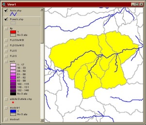
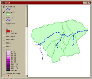
Figure 9: Sub-system extraction by selecting all the relevant sub-basin
polygons. Upstream reaches are selected to help identify system sources.
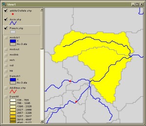
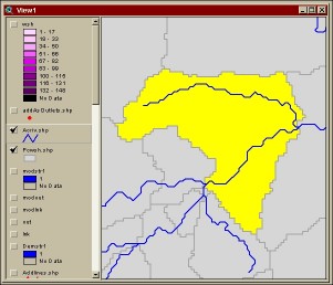
The second method is less flexible, but easier to implement. After manually selecting the downstream sub-basin polygon, it automatically identifies and selects all the sub-basin polygons located upstream, and consequently does not support the use of inlets. Reach polylines contained within the selected polygons are selected automatically. This method is convenient when dealing with a significant number of polygons in the study area. Figure 10 shows a sub-system extraction when only the most downstream polygon is manually selected.
Figure 10: Sub-system extraction by selecting the downstream sub-basin
polygon, and automatically selecting all other upstream polygons.
Topologic Analysis and Preparation of HEC-HMS Basin File
Establishing the topology of the hydrologic system consists of determining the element located downstream of each element. Since the HEC-HMS hydrologic schematic allows only one downstream element, no ambiguity is introduced in this process. After establishing the system topology based on the sub-basin and reach data sets, an ASCII file -- readable by HEC-HMS -- is used to record the type (i.e., sub-basin, reach, source, sink, reservoir or junction), hydrologic parameters, and downstream element of each hydrologic element of the system. A background map file -- also readable by HEC-HMS -- is used to graphically represent sub-basins and reaches, and ease the identification of hydrologic elements. These files constitute the input to the basin component of HEC-HMS. Figure 11 shows three different sections of the basin file.
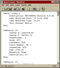
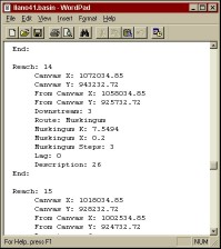
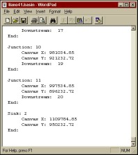
Figure 11: HEC-HMS basin file in ASCII format. Hydrologic parameters calculated
in GIS and stored in the attribute tables are transferred to the basin
file.
This basin file, when opened with HEC-HMS, generates a topologically correct schematic network of hydrologic elements and displays it in the HEC-HMS - Schematic window together with the background map. Figure 12 shows a detail of an HEC-HMS schematic and the corresponding sections of the basin file used to build it. Figure 13 shows the HEC-HMS – Schematic window after opening the basin file.
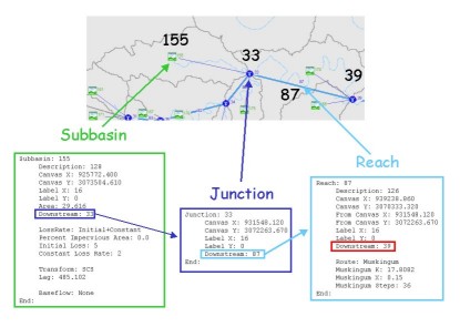
Figure 12: HMS schematic of the hydrologic system constructed from the
basin file.
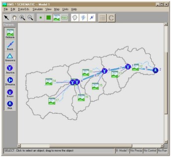
Figure 13: HEC-HMS display of the schematic of the hydrologic system
as described by basin input component.
The process of generating input data for the precipitation component consists of calculating precipitation time series for sub-basin polygons from precipitation time series at precipitation gages or precipitation cells (i.e., NEXRAD cells). At present, two precipitation methods are supported by CRWR-PrePro: (1) user-specified gage weighting, and (2) GridParm. Automatic determination of user-specified gage weights for precipitation interpolation, based on Thiessen and sub-basin polygon data sets, was developed by Dugger (1997). Precipitation time series at sub-basins are estimated as an area-weighted average of precipitation time series at gages. GridParm (HEC 1996), as mentioned above, was originally developed at HEC in Arc Macro Language (AML) and rewritten at CRWR as an Avenue script. GridParm (short for grid cell parameters) is used to determine parameters of precipitation cells for use with the ModClark sub-basin routing method of HEC-HMS.
User-Specified Gage Weighting
Sub-basin precipitation time series are calculated as the weighted average of gage precipitation time series. For this purpose, a set of weights that capture the relative importance of the precipitation at each gage on the precipitation of each sub-basin is calculated. Precipitation time series at the gages are stored in Data Storage System (DSS) format (HEC 1995). Figure 14 shows precipitation data in text format.
Figure 14: Precipitation data in text format before using HEC-DSS to
convert it into DSS format.
Given a set of points that represent gages for which precipitation time series are known, Thiessen polygons are used to establish the area of influence of each precipitation gage. Thiessen polygons are constructed by drawing perpendiculars at the midpoints of the segments that connect the gages, so that all points within a polygon are closer to the polygon gage than to any other gage. By intersecting the Thiessen with the sub-basin polygons, a new set of smaller polygons is defined in such a way that each new polygon is related to one (and only one) Thiessen polygon and one (and only one) sub-basin polygon. Figure 15 shows the polygons resulting of the intersection of Thiessen polygons and sub-basin polygons.
Figure 15: Intersection of sub-basin polygons with Thiessen polygons.
Red dots indicate precipitation drainage gages.
The ratio of the area of a new polygon to the area of its corresponding sub-basin polygon represents the weight of the gage for the sub-basin. This can also be expressed as
![]() ( 5 )
( 5 )
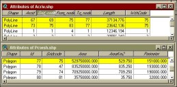
where Aij is the area of the polygon generated by intersecting sub-basin j with the Thiessen polygon of gage i, Sj is the area of sub-basin j, and wij is the weight of gage i for sub-basin j. The sum of the weights of a sub-basin should add up to one. In Figure 16, the three selected polygons originally formed a complete sub-basin, and their weight is proportional to their area.
Figure 16: Intersection of a sub-basin polygon with the Thiessen polygons.
In the table below, the area of each of the yellow polygons is stored in
the field Area, the sub-basin area in the field WtshdArea,
and the weights (the ratio of these two areas) in the field %WshArea
After establishing the weight values based on the sub-basin and Thiessen polygon data sets, an ASCII file -- readable by HEC-HMS -- is used to record the gage and sub-basin information. The gage information consists of the gage name, location, type (i.e., incremental or cumulative), and reference to the precipitation time series in the DSS file. The sub-basin information consists of the sub-basin name or identification code, and the name of each gage with its corresponding weight. Figure 17 shows the HEC-HMS precipitation weights text file.
Figure 17: HEC-HMS precipitation weights file in ASCII format. Gage
weigths calculated in GIS and stored in the attribute tables are transferred
to the precipitation weights file.
Finally, the sub-basin precipitation time series are calculated by HEC-HMS as
![]() ( 6 )
( 6 )
where pi(t) is the precipitation time series at gage i, and Pj(t) is the precipitation time series at sub-basin j.
GridParm
GridParm (short for grid cell parameters) is used to determine parameters of precipitation cells for use with the ModClark sub-basin routing method of HEC-HMS. ModClark, a variation of the Clark unit-hydrograph model (Clark 1945), has been developed by HEC for HEC-HMS as a sub-basin routing option suitable to support NEXRAD precipitation data. In the ModClark method, the drainage area is subdivided into elementary cells in which precipitation is uniform and known, and the hydrograph is calculated as the sum of the contribution of each cell (or fraction of cell) within the sub-basin. Although cells are usually rectangular since the method was developed to support NEXRAD precipitation data, no restriction on the cell shape exists. Calculation of the routing parameters, area and flow distance to the outlet, to track the water from the precipitation cell to the outlet is done by GridParm.
To calculate these parameters, three data sets are defined: (1) sub-basin polygons, (2) precipitation cell polygons, and (3) flow-length downstream to the sub-basin outlet grid. Sub-basin polygons are intersected with precipitation cell polygons yielding a new set of polygons, which are complete cells in case they were completely within a sub-basin, or fractions of cells in case they were partially contained by two or more sub-basins. Each of these new polygons is called GridCell, and is related to one (and only one) sub-basin polygon. The average distance from the GridCell to the sub-basin outlet is calculated as the mean of the flow-length grid values within the GridCell. Figure 18 shows the intersection of precipitation cells with sub-basin polygons.
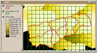
Figure 18: Intersection of precipitation cells with sub-basin polygons.
The flow-length to the sub-basin outlet grid is displayed as background.
After establishing the GridCell parameters, an ASCII file -- readable by HEC-HMS -- is used to record the sub-basin and GridCell information. The sub-basin information consists of the sub-basin name. The GridCell information consists of the location, area and distance to the sub-basin outlet. Figure 19 shows the text file with GridCell parameters as prepared by GridParm.
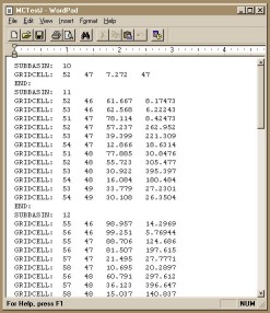
Figure 19: ASCII file with precipitation cell parameters for use with
the ModClark sub-basin routing method.
A connection between GIS data sets describing a hydrologic system and HEC's Hydrologic Modeling System (HEC-HMS) has been developed and called CRWR-PrePro.
CRWR-PrePro extracts topographic, topologic and hydrologic information from digital spatial data, and prepares an input file for the basin component of HEC-HMS, which when opened automatically creates a topologically correct schematic network of sub-basins and reaches, and attributes each element with selected hydrologic parameters. CRWR-PrePro also generates an input file for the precipitation component of HEC-HMS. Two methods to interpolate precipitation records are supported: Thiessen polygons to calculate average precipitation at the sub-basins, and GridParm to calculate routing parameters of the precipitation cells for use with the ModClark sub-basin routing method.
At the moment, CRWR-PrePro calculates or imports parameters for: the Soil Conservation Service (SCS) curve number method and the initial plus constant loss method for loss rate calculations; the SCS unit hydrograph model for sub-basin routing for which the lag-time can be calculated with the SCS lag-time formula or as a fraction of the length of the longest channel divided by the flow velocity; and the Muskingum method and the lag method for flow routing in the reaches (depending on the reach length).
Using CRWR-PrePro, the determination of physical parameters for HEC-HMS is a simple and automatic process that accelerates the setting up of a hydrologic model and leads to reproducible results.
Development of CRWR-PrePro has been funded by the Texas Department of Transportation (TxDOT) and the Hydrologic Engineering Center (HEC) of the United States Army Corps of Engineers. The contribution of Joaquim Pinto da Costa at the Instituto da Agua (INAg) of Portugal is appreciated.
Asquith, W., and R. Slade (1997), Regional Equations for Estimation of Peak Streamflow Frequency for natural Basins in Texas, USGS Water-Resources Investigations Report 96-4307, Austin, TX.
Clark, C.O. (1945), Storage and the Unit Hydrograph, Trans. Am. Soc. Civ. Eng., ASCE, Vol 110, pp.1419-1488.
Djokic, D., Ye, Z., and Miller, A. (1997), Efficient Watershed Delineation Using ArcView and Spatial Analyst, Proc. 17th Annual Esri User Conference, San Diego, CA.
Dugger, A. (1997), Linking GIS with the Hydrologic Modeling System: An Investigation of the Midwest Flood of 1993, Masters Report, Department of Civil Engineering, University of Texas at Austin, TX.
Esri (1992), Cell-based Modeling with Grid 6.1: Supplement - Hydrologic and Distance Modeling Tools, Environmental Systems Research Institute, Redlands, CA.
Esri (1997), Watershed Delineator Application - User's Manual, Environmental Systems Research Institute, Redlands, CA.
HEC (1990), HEC-1 - Flood Hydrograph Package - User's Manual, Hydrologic Engineering Center, U.S. Army Corps of Engineers, Davis, CA.
HEC (1995), HEC-DSS - User's Guide and Utility Manuals, Hydrologic Engineering Center, U.S. Army Corps of Engineers, Davis, CA.
HEC (1996), GridParm - Procedures for Deriving Grid Cell Parameters for the ModClark Rainfall-Runoff Model - User's Manual, Hydrologic Engineering Center, U.S. Army Corps of Engineers, Davis, CA.
Hellweger, F., and D.R.Maidment (1999), Definition and Connection of Hydrologic Elements Using Geographic Data, ASCE – Journal of Hydrologic Engineering, Vol. 4, No. 1.
Jensen, S.K., and J.O. Domingue (1988), Extracting Topographic Structure from Digital Elevation Data for Geographic Information System Analysis, Photogrammetric Engineering and Remote Sensing 54 (11).
Jensen, S.K. (1991), Applications of Hydrologic Information Automatically Extracted from Digital Elevation Models, Hydrological Processes 5(1).
Maidment, D.R. (1992), Grid-based Computation of Runoff: A Preliminary Assessment, Hydrologic Engineering Center, US Army Corps of Engineers, Davis, CA.
Olivera, F., J. Bao and D.R. Maidment (1997), Geographic Information System for Hydrologic Data Development for Design of Highway Drainage Facilities, Research Report 1738-3, Center for Transportation Research - University of Texas at Austin, TX.
Olivera, F. and D.R. Maidment (1998a), HEC-PrePro v. 2.0: An ArcView Pre-Processor for HEC’s Hydrologic Modeling System, Proceedings of the 18th Esri Users Conference, San Diego, CA.
Olivera, F. and D.R. Maidment (1998b), GIS for Hydrologic Data Development for Design of Highway Drainage Facilities, Transportation Research Record # 1625, pp. 131-138, Transportation Research Board, Washington DC.
Smith, P. (1995), Hydrologic Data Development System, Masters Thesis, Department of Civil Engineering, University of Texas at Austin, TX.
Soil Conservation Service (1972), National Engineering Handbook - Section 4: Hydrology, U.S. Department of Agriculture, Washington DC.
USGS a, 7.5-Minute Digital Elevation Model Data, http://edcwww.cr.usgs.gov/glis/hyper/guide/7_min_dem as of July 6, 1999.
USGS b, 1-Degree Digital Elevation Models, http://edcwww.cr.usgs.gov/glis/hyper/guide/1_dgr_dem as of July 6, 1999.
USGS c, Global 30 arc-second Elevation Data Set, http://edcwww.cr.usgs.gov/landdaac/gtopo30/gtopo30.html as of July 6, 1999.
Francisco
Olivera, PhD
Research Scientist
University of Texas at Austin - Center for Research in Water Resources
J.J.Pickle Research Campus # 119 - Austin, TX 78712
Telephone: (512) 471-0570 - FAX: (512) 471-0072
folivera@mail.utexas.edu
David Maidment,
PhD
Professor of Civil Engineering
University of Texas at Austin - Center for Research in Water Resources
J.J.Pickle Research Campus # 119 - Austin, TX 78712
Telephone: (512) 471-0065 - FAX: (512) 471-0072
maidment@mail.utexas.edu