Abstract

Topography plays an important role in the distribution and flux of water and energy within natural landscapes. The automated extraction of topographic parameters from DEMs is recognized as a viable alternative to traditional surveys and manual evaluation of topographic maps, particularly as the quality and coverage of DEM data increases. The capabilities and limitations of DEMs for use in water resources model applications are reviewed. Specifically, data availability, quality and resolution are discussed from an application perspective. Issues related to the automated extraction of topographic and drainage information from DEMs are presented. These include the identification of drainage in the presence of pits and flat areas in the DEM, the determining role of channel source definition in drainage network configuration, and network analysis capabilities for raster networks. Findings on the latest research results regarding the reduction of distributed subcatchment properties into a representative value for the subcatchments are also presented. Increasing quality and resolution of DEM products, new raster processing methodologies and expanding GIS capabilities and linkages with water resources models are expected to lead to a heavier reliance on DEMs as a source of topographic and surface drainage information.

Introduction

Hydrologic process and water resource issues are commonly investigated by use of distributed watershed models. These watershed models require physiographic information such as configuration of the channel network, location of drainage divides, channel length and slope, and subcatchment geometric properties. Traditionally, these parameters are obtained from maps or field surveys. Over the last two decades this information has been increasingly derived directly from digital representations of the topography (Jenson and Domingue, 1988; Mark, 1984; Moore et al., 1991; Martz and Garbrecht, 1992). The digital representation of the topography is called a Digital Elevation Model (DEM). The automated derivation of topographic watershed data from DEMs is faster, less subjective and provides more reproducible measurements than traditional manual techniques applied to topographic maps (Tribe, 1992). Digital data generated by this approach also have the advantage that they can be readily imported and analyzed by Geographic Information Systems (GIS). The technological advances provided by GIS and the increasing availability and quality of DEMs have greatly expanded the application potential of DEMs to many hydrologic, hydraulic, water resources and environmental investigations (Moore et al., 1991). In this paper the production, availability, quality, resolution and capabilities of DEMs are reviewed and discussed with respect to the derivation of topographic data in support of hydrologic and water resources investigations. The subject matter covered in this paper pertains to DEMs of natural landscapes and does not extend to urbanized settings where small-scale and man made structures such as street gutters, inlets, drainage ditches and culverts control surface drainage patterns.

DEM production, quality and availability

The most common DEM data structure is the raster or grid structure. These normally consist of a matrix of square grid cells with the mean cell elevation stored in a two dimensional array. Location of a cell in geographic space is implicit from the row and column location of the cell within the array, provided that the boundary coordinates (geo-references) of the array are known. Grid DEMs are widely available and used because of their simplicity, processing ease and computational efficiency (Martz and Garbrecht, 1992). Disadvantages include grid size dependency of certain computed topographic parameters (Fairfield and Leymarie, 1991) and inability to locally adjust the grid size to the dimensions of topographic land surface features. Other DEM data structures, such as the Triangulated Irregular Network and contour-based structures, have overcome some of the disadvantages of grid DEMs, however they have shortcomings of their own and are not as widely available and used as grid DEMs. The remainder of this paper will focus on the popular grid-type DEMs.

DEMs produced by the USGS are classified into three levels of increasing quality. Level 1 classification is generally reserved for data derived from scanning National High-Altitude Photography Program, National Aerial Photography Program, or equivalent photography. A vertical Root Mean Square Error (RMSE) of 7 meters is the targeted accuracy standard, and a RMSE of 15 meters is the maximum permitted. Level 2 classification is for elevation data sets that have been processed or smoothed for consistency and edited to remove identifiable systematic errors. A RMSE of one-half of the original map contour interval is the maximum permitted. There are no errors greater than one contour interval in magnitude. Level 3 classification DEMs are derived from Digital Line Graph (DLG) data by using selected elements from both hypsography (contours, spot elevations) and hydrography (lakes, shorelines, drainage). If necessary, ridge lines and major transportation features are also included in the derivation. A RMSE of one-third of the contour interval is the maximum permitted. There are no errors greater than two-thirds of the contour interval in magnitude. Most data produced within the last decade fall into the level 2 classification. The availability of level 3 DEMs is very limited.

The USGS, Earth Science Information Center, Reston, Virginia, offers a variety of digital elevation data products (USGS, 1990). Other sources for DEM data include the former Defense Mapping Agency (DMA) (now the National Imagery and Mapping Agency, NIMA), and the National Geophysical Data Center (NGDC) of the National Oceanic and Atmospheric Administration (NOAA). Custom DEM data can also be obtained through a number of commercial providers. New technologies, such as Laser Altimetry (LA) (Ritchie, 1995) and Radar Interferometry (RI) (Zebker and Goldstein, 1986), are currently being explored for production of global high quality and high resolution DEMs (Gesch, 1994).

DEM accuracy considerations in water resource applications

DEMs are used in water resources projects to identify drainage related features such as ridges, valley bottoms, channel networks and surface drainage patterns, and to quantify subcatchment and channel properties such as size, length, and slope. The accuracy of this topographic information is a function both of the quality and resolution of the DEM, and of the DEM processing algorithms used to extract this information.

The suitability of a USGS DEM for water resources projects depends largely on the DEM production techniques. USGS 7.5 minutes DEMs produced before 1988 were mainly based on manual profiling of photogrammetric stereo-models (USGS, 1990). In low relief landscapes, the resulting DEMs often display systematic east-west striping patterns that can make them unsuitable for parameterization of drainage features (Garbrecht and Starks, 1995). Figure 1a shows two adjacent DEMs that were produced by different techniques. The left side illustrates the east-west striping pattern associated with the manual profiling of photogrammetric stereo-models. The impact of the striping on drainage studies is threefold. First, the outlines of drainage features, such as depressions or drainage paths, are not well defined. Boundaries of shallow features that have a north-to-south orientation (i.e. perpendicular to the striping) are often represented in the DEM as ragged lines having east-to-west indentations. Second, drainage paths are systematically biased in the east-to-west direction because of flow draining into and following the artificial elevation stripes. Figure 1b illustrates the differences in drainage pattern as a result of the striping pattern in the elevation data. And, third, the striping may introduce drainage blockages in the north-to-south flow component. These drainage blockages can produce artificial depressions of varying sizes. The source of the striping is a combination of human and algorithmic errors associated with the manual profiling method (B. Kunert, USGS, Rolla, Mid Continent Mapping Center, personal communication). While these "striping" errors are well-recognized (Garbrecht and Starks, 1995), they are within the accuracy standards of the USGS (1990). While most of the DEMs being developed today are derived from DLG and are processed to Level 2 standards, many of the DEMs being distributed today were developed in the past and only meet Level 1 standards.

Figure 1a: Coverage of two adjacent USGS 7.5 minute DEMs near Amarillo, Texas; DEM elevation values in gray scale.

Figure 1b: Coverage of two adjacent USGS 7.5 minute DEMs near Amarillo, Texas; DEM elevation values in gray scale with GIS derived drainage network.

Level 1 standards demand a RMSE value of 7 meters, with a maximum permitted value of 15 meters. An absolute elevation error tolerance of 50 meters is set for blunders for any grid node when compared to the true height from mean sea level. Also, any array of 49 contiguous elevation points shall not be in error by more than 21 meters (USGS, 1990). These tolerances in elevation are large for drainage investigations since an elevation difference of 1 or 2 meters can affect flow path and runoff characteristics.

DEM horizontal resolution and its ratio to vertical resolution can have a significant bearing on computed land surface parameters that involve differences in elevations. For example, slope is computed as the difference in elevation between two adjacent pixels divided by the distance between them. Since DEM elevations are generally reported in full meters or feet, the computed slope can only take on a limited number of discreet values. For a 30 meter DEM with elevations reported in meters, a slope value between two pixels can be zero (no change in elevation), 0.033 (1 meter change in elevation), or a multiple thereof. Such increments may be adequate to represent slope values in mountainous terrain, but for flat areas, such as the Great Plains of the United States, a 1 meter vertical DEM resolution is insufficient to provide accurate local slope values. Thus, DEMs of low relief landscape and limited vertical resolution do not lend themselves well to an accurate determination of drainage slopes and precise location of channels and ridges. The problems of DEM quality and resolution can generally not be overcome by smoothing or averaging the DEM. Such approaches simply cover up the problems without increasing the quality of the output. The easiest solution to overcome the described resolution problems is to custom produce a DEM with a pre-specified horizontal to vertical resolution ratio, or to use a high resolution DEM produced by more advanced methods. Other solutions include the use of DEM analysis methods that are designed to overcome problems associated with digital representations of low relief landscapes by DEMs of limited resolution (Garbrecht and Martz, 1999a). Examples of such problems are the increased occurrence and size of flat areas and spurious pits. Pits are cells that have no adjacent cell at a lower elevation and, consequently, have no downslope flow path to an adjacent cell. On the other hand, flat areas are characterized by adjacent cells with same elevation values. Pits and flat areas occur in most raster DEMs, but are predominant in limited resolution DEMs of low relief landscapes. Figure 2 shows the spatial distribution and extent of pits and flat areas (areas in light gray) of a DEM of a watershed in Central Oklahoma. The predominance of pits and flat areas in the valley bottoms (low relief areas) are clearly visible. Pits are usually viewed as spurious features that arise from interpolation errors during DEM generation and truncation of interpolated values on output (O’Callaghan and Mark, 1984; Mark, 1988; Fairfield and Leymarie, 1991). Pits are a major difficulty for DEM evaluation methods that rely on the overland flow simulation approach to drainage analysis because a lack of downslope flow paths leads to incomplete drainage pattern definition. The drainage identification problems for flat areas are similar to those encountered for pits. This subject is addressed in greater depth in the section on automated extraction of drainage features from DEMs.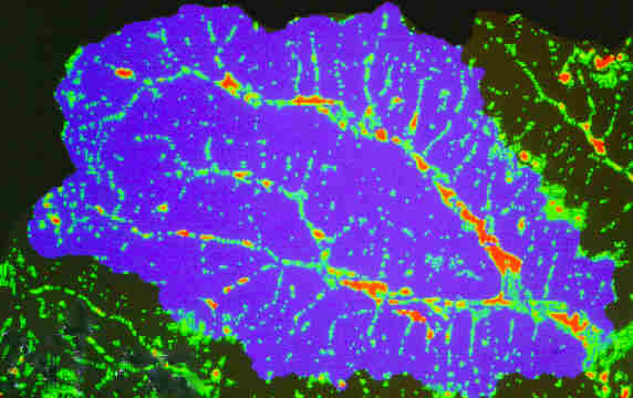

Figure 2: Spatial distribution and extent of pits and flat areas in a DEM of a watershed in Central Oklahoma.

DEM selection criteria

Both quality and resolution must be considered in the selection of a DEM for hydrologic modeling. Quality refers to the accuracy of the elevation data while resolution refers to the precision of the data; specifically to the horizontal grid spacing and vertical elevation incrementation. Quality and resolution must be consistent with the scale and model of the physical process under consideration and with the study objectives. For many applications of physical-process based environmental models, the USGS 30 by 30 meter DEM data (Level 1 and 2) has broad accuracy standards and a rather coarse resolution with documented shortcomings (Garbrecht and Starks, 1995; Ostman, 1987; Topographic Science Working Group, 1988). In particular, surface drainage identification is difficult in low relief landscapes, as is derivation of related information such as slope and landform curvature. Research is underway to assess the impact of accuracy limitations, noise and low resolution of DEM data on modeling results. Examples of such studies include Wolock and Price (1994) and Zhang and Montgomery (1994).

The accuracy of drainage features extracted from DEMs as a function of DEM resolution was investigated by Garbrecht and Martz (1994). The horizontal resolution of a DEM with an original grid spacing of 30 meters was decreased by cell aggregation. Selected drainage features for several hypothetical channel network configurations were extracted for a range of DEM resolutions using the TOPAZ software (Garbrecht and Martz, 1994). Figure 3 illustrated the loss of accuracy from left to right with increasing grid coefficient. The grid coefficient is the area of a cell divided by the network reference area, which is the mean subcatchment area. The values shown are for selected network features such as channel source area, number of channels, channel length, drainage density, etc. The sensitivity analysis suggested that a DEM should have a grid area less than 5% of the network reference area to reproduce the selected drainage features with an accuracy of about 10%. It was concluded that the grid resolution dependency was introduced by the inability of a DEM to accurately reproduce drainage features that are at the same scale as the spatial resolution of the DEM. For sinuous channels, this results in shorter channel lengths and for networks with high drainage density, it leads to channel and drainage area capturing. Channel and drainage area capturing occurs when the DEM resolution can no longer resolve the separation between channels or drainage boundaries. In such situations, the number of channels, the size of direct drainage areas, and the channel network pattern may depart considerably from the one obtained by a high resolution DEM. Thus, if small drainage features are important, the resolution must be selected relative to the size of these features.

Figure 3: Departures from reference for selected drainage features versus grid coefficients (from Garbrecht and Martz, 1994)

Zhang and Montgomery (1994) used high-resolution digital elevation data from two small catchments in the western United States to examine the effect of DEM resolution on the portrayal of the land surface and results of hydrologic simulations. They evaluated DEMs that had resolutions of 2 through 90 meters and concluded that grid sizes of 10 meters would suffice for many DEM-based applications of geomorphic and hydrologic modeling. Commenting on this research, Garbrecht and Martz (1996) suggested that the selection of DEM resolution for simulation applications depends not only the scale of the processes being modeled, but also in the numerical simulation approach and the specific landscape parameters that are to be extracted from the DEM. For hydrologic models that operate on a grid approach, landscape parameters and simulation processes are determined at every grid cell. Hence, the data volume and computational resources are proportional to the number of grid cells which themselves increase quadratically for each doubling of the horizontal DEM resolution. This can be a limiting factor for practical applications and encourages the selection of lower resolution DEM. On the other hand, models that use subcatchments as their operating unit depend only on the DEM to extract representative parameters for the entire subcatchment, and the processes are simulated at the subcatchment level, independently of DEM resolution. This approach is less demanding with regard to data volume and computational resources. It often is also less sensitive to DEM noise and resolution because representative landscape parameters for subcatchments, such as hillslope length, width and slope are derived from many grid cells. As a result the effects of grid induced local variability and discrete incrementation are largely eliminated by the averaging process over the subcatchment.

In a study by Seybert (1996), GIS coverages of land use, soils and elevation (DEM) were used to study the effect of spatial data resolution degradation on the output of an event based surface runoff model. The study was performed on a 7.27 km² (2.81 mi²) agricultural watershed in central Pennsylvania. Square cell dimensions ranging from 5 meters to 500 meters were investigated, beginning with spatial data layers of the finest resolution and systematically degrading the data to the coarsest resolution. Results of the spatial data resolution study indicate that volume estimates in the model are less sensitive to spatial resolution change than peak flow estimates. Also, increasing the number of subcatchments in the watershed representation caused the model to increase estimates of runoff volume and peak flow. The ratio of average subcatchment area to grid cell area was used as an indicator of spatial resolution and an overall catchment to grid ratio of about 10² was found to be an acceptable threshold of spatial resolution for reasonable model results.

The above discussion provides some broad indications as to appropriate DEM resolutions for specific applications, but there appears to be no guidelines for DEM resolution for general applications. In theory, the DEM resolution should be selected as a function of the size of the land surface features that are to be resolved, the scale of the processes that are modeled and numerical model used to model the processes. In practice, however, the selection of DEM resolution for a particular application is often driven by data availability, judgement, test applications, experience and, last but not least, cost.

Automated extraction of drainage features

The major issues with the derivation of surface drainage, drainage networks and associated topologic information from DEMs are related to the resolution and quality of the DEM and to the methodology used to derive this information. Issues of DEM resolution and quality have been addressed in an earlier section. This section addresses the raster processing methodology used in the derivation of the topographic/topologic drainage information from USGS DEMs. Discussions are limited to methodologies based on the D-8 method (described below). The D-8 method is selected here because it is a simple and widely used raster DEM processing method.

The D-8 method (Fairfield and Leymarie, 1991) defines the drainage network from raster DEMs using an overland flow analogue. The method identifies the steepest downslope flow path between each cell of a raster DEM and its eight neighbors (hence the name D-8 method), and defines this path as the only flow path leaving the raster cell. The drainage network is identified by selecting a threshold catchment area at the bottom of which a source channel originates; all cells with a catchment area greater than this threshold catchment area as classified as part of the drainage network. This drainage network identification approach is simple and directly generates connected networks (Martz and Garbrecht, 1992). The use of the D-8 method for catchment area and drainage network analysis recently has been criticized on the grounds that it permits flow only in one direction away from a DEM cell. This fails to represent adequately divergent flow over convex slopes (Freeman, 1991; Quinn et al., 1991; Costa-Cabral and Burges, 1994) and can lead to a bias in flow path orientation (Fairfield and Leymarie, 1991). Although the multiple flow direction algorithm seems to give superior results in the head-water region of a source channel, a single flow-direction algorithm is superior in zones of convergent flow and along well-defined valleys (Freeman, 1991; Quinn et al., 1991). Thus, for overland flow analysis on hillslopes the multiple flow approach may be more appropriate. However, if the primary objective is the delineation of the drainage network for large drainage areas with well-developed channels, the use of a single flow-direction algorithm seems more appropriate (Martz and Garbrecht, 1992).

The D-8 method, as well as many other approaches, has difficulties identifying surface drainage in the presence of depressions, flat areas and flow blockages (Garbrecht and Starks, 1995; Martz and Garbrecht, 1998). These features are often the result of data noise, interpolation errors and systematic production errors in DEM elevation values. Such features occur in most DEMs and are viewed as spurious, mainly because of their predominantly numerical origin. The difficulties arise from the fact that raster cells in depressions, sinks and flat areas have no neighboring cells at a lower elevation, and, consequently, have no downslope flow path to a neighbor cell. It is common practice to remove the depressions and flat areas prior to drainage identification.

Surface Drainage Identification from Raster DEMs

A number of methods have been developed for treating sinks and flat areas in DEMs for automated analysis of hydrographic terrain features. Band (1986) simply increases the elevation of sink cells until a downslope path to a cell becomes available, under the constraint that flow may not return to a sink cell. O’Callaghan and Mark (1984) suggest smoothing a DEM prior to analysis to reduce the size and number of sinks. Both Jenson and Domingue (1988) and Martz and De Jong (1988) provide methods for treating sinks in a more general and effective manner (Freeman, 1991). These methods cope with complex topographic situations such as nested depressions, depressions with flat areas, and truncated depressions and flat areas at the edge of the DEM. They involve "filling" each depression in the DEM to the elevation of the lowest overflow point out of the sink. This approach implies that all sinks are the result of underestimation of elevation (Martz and Garbrecht, 1998). However, some sinks arise from obstruction of flow paths by overestimated elevations. In such cases, breaching the obstruction is more appropriate than filling the sink created by the obstruction (Martz and Garbrecht, 1999a). Obstruction breaching is particularly effective in DEMs of landscapes that have a low relief relative to the vertical resolution of the DEM because sinks caused by flow path obstruction are more prevalent in these situations. A combined filling and breaching method was presented by Garbrecht et al. (1996).

Once the sinks in a DEM are removed by breaching and filling, the resulting flat surface must still be interpreted to define the surface drainage pattern. Flat surfaces do not only result from sink filling, but can also result from too low a vertical and/or horizontal DEM resolution to adequately represent the landscape, or from truly flat landscape (which seldom occurs). Several approaches for defining surface drainage across flat areas have been discussed earlier (Band, 1986; Jenson and Domingue, 1988; Martz and De Jong, 1988). Other methods rely on techniques ranging from landscape smoothing to arbitrary flow direction assignment. A discussion of various approaches can be found in Tribe (1992) and subsequent comments by Martz and Garbrecht (1995). A more recent approach has been presented by Garbrecht and Martz (1995). This approach is based on the recognition that surface drainage in natural landscapes is towards lower terrain and away from higher terrain. To reproduce such a trend on a flat surface, two shallow gradients are imposed on flat surfaces to force flow away from higher terrain surrounding the flat surface and attracting flow towards lower terrain on the edge of the flat surface. This approach results in a convergent flow direction pattern over the flat surface that is also consistent with the topography surrounding the flat surface (Garbrecht et al., 1996). Figure 4a show the drainage pattern of a hypothetical mountain saddle situation which consists of a flat surface at the center between higher terrain to the right and left, an three locations of lower terrain, one at the top and two at the bottom. The computed drainage, as well as flow convergence and consistency with the surrounding terrain configuration, is a great improvement over drainage patterns from methods that are plagued by the parallel flow problem (Figure 4b). It must, however, be recognized that any method of drainage identification in flat areas is an approximation and may not accurately reflect the actual drainage pattern which may follow channel incisions that are to small to be resolved at the resolution of the digital landscape.

Figure 4a: Computed drainage pattern over a flat saddle topography (from Garbrecht and Martz, 1997b). Arrows indicate drainage direction; arrow size is representative of upstream drainage area; drainage divides are indicated by heavy lines; drainage computed after Garbrecht and Martz (1996).

Figure 4b: Computed drainage pattern over a flat saddle topography (from Garbrecht and Martz, 1997b). Arrows indicate drainage direction; arrow size is representative of upstream drainage area; drainage divides are indicated by heavy lines; drainage computed after Martz and De Jong (1988) and Jenson and Domingue (1988).

Drainage network extraction

A drainage network can be extracted from a DEM with an arbitrary drainage density or resolution (Tarboton et al., 1991). The characteristics of the extracted network depend on the definition of channel sources on the digital land surface topography. Once the channel sources are defined, the essential topology and morphometric characteristics of the drainage network are implicitly defined because of their close dependence on channel source definition. Thus, the proper identification of channel sources is critical for extraction of a representative drainage network from DEMs.

The fundamental concepts that deal with channel initiation can readily be found in the scientific literature (Montgomery and Dietrich, 1988, 1989 and 1992). Two prevailing methods for network sources in DEMs are the constant threshold area and the slope-dependent critical support area method (Montgomery and Foufoula-Georgiou, 1993; Tribe, 1992). The constant threshold area method assumes that channel sources represent the transition between the convex profile of the hillslope (sheet flow dominated) and the concave profiles of the channel slope (channel discharge dominated). The constant threshold area method has found widespread application (Band, 1986; Morris and Heerdegen, 1988; Tarboton et al., 1991; Gardner et al., 1991). The application details, use and implications of this method are discussed by Tarboton et al. (1991) and Montegomery and Foufoula-Georgiou (1993). Garbrecht and Martz (1995) broadened the use of the constant threshold area method by allowing the threshold area to vary within the DEM. This is particularly useful in large watersheds in which geology and drainage network characteristics display distinct spatial patterns. The user must, however, establish a priori the values of the constant threshold areas and their region of application.

The slope-dependent critical support area method assumes that the channel source represents an erosional threshold. This assumption implies that the channel source is the result of a change in sediment transport processes from sheet flow to concentrated flow, rather than a spatial transition in longitudinal slope profiles. This method was presented by Montgomery and Foufoula-Georgiou (1993) and is based on the channel initiation work by Dietrich et al. (1993). The main differences between the networks defined by the constant and slope-dependent thresholds support area methods are the spatial variability of the slope. Montgomery and Foufoula-Georgiou (1993) report that with the slope-dependent threshold method, drainage density is greater in steeper portions of the catchment, as is found in natural landscapes.

The constant threshold area method appears more practical in application, as is apparent by its widespread use. The current preference for this method can be attributed to the fact that local slope values are difficult to obtain from DEMs. Indeed, a DEM with horizontal and vertical resolution of 30 m and 1 meter, respectively, can only produce local slopes of zero, 0.03 or increments thereof. Thus, an accurate estimation of local slope requires either a high-resolution DEM or field measurements.

Another issue that is often of concern with drainage networks extracted from DEMs is the precise positioning of channels in the digital landscape. Comparisons with actual maps or areal photos often show discrepancies, particularly in low-relief landscapes. The primary reason for this discrepancy is the approximate nature of digital landscapes that cannot capture important topographic information that is below the DEM resolution. Though the channel position in the digital landscape is consistent with the digital topography, it may not reflect the actual drainage path in the field. From a practical point of view, this dilemma can be overcome by "burning in" the path of the channels along pre-digitized pathways. This is achieved by artificially lowering the elevation of the DEM cells along digitized lines or raising the entire DEM except along stream paths (Cluis et al., 1996; Maidment et al., 1996). However, caution is advised with this method because it may produce flow paths that are not consistent with the digital topography.

Drainage network topology

Once a channel network is extracted from a DEM, it is usually displayed as a string of raster cells. For these images to be useful in hydrologic and runoff modeling, individual channel links and adjacent contributing areas must be explicitly identified and associated with topologic information for upstream and downstream connections. Such channel indexing is straightforward in vector GIS, but usually not easy in raster data. Yet, the spatial organization and connectivity of the channel network is fundamental for flow routing and automated linkage of raster GIS information of the network and traditional surface runoff modeling. Garbrecht and Martz (1997a) have proposed an algorithm that interprets a GIS raster image of a network, indexes the channel links and network nodes, and organizes the channels into a sequence for cascade flow routing (Garbrecht, 1988). The algorithm uses a cell-by-cell trace along the channels of the network to identify for each channel link the Strahler order, the index, the sequence for cascade flow routing, the upstream inflow tributaries, the downstream connection, and the channel longitudinal slope and length. This data is provided in tabular format and can be used as input data for hydrologic modeling.

Calculation of distributed subcatchment properties

The traditional automated extraction of drainage features from DEMs has focused on the identification of drainage boundaries, channels and watershed segmentation (Band, 1986; Jenson and Domingue, 1988; Martz and Garbrecht, 1992; Wolock and McCabe, 1995; Tarboton et al. 1991). The identification of distributed properties for subcatchments from Digital Elevation Models (DEM) is a relatively recent area of exploration. Contrary to the uniquely identifiable topographic features such as drainage divides and channels, distributed properties require a method or model to reduce the distributed information into a representative value for the entire subcatchment. Thus, a representative subcatchment property can have different values depending on the underlying model used for data reduction. The discrepancies between the different values are not approximation errors, but result from the different interpretations of the subcatchment property by the data reduction models. These differences can have significant implications for distributed rainfall-runoff and erosion modeling. In the following alternative models for subcatchment length and slope calculations, as well as the resulting differences in the representative length and slope values, are discussed, and recommendations for proper application of the various alternatives are proposed. The alternative data reduction models are compatible with the assumptions of the D-8 method since all calculations are performed on DEM properties derived by that method.

Subcatchment length alternatives

A subcatchment is a hillslope area that drains overland flow into the first adjacent downslope channel. Subcatchment length is often needed to estimate runoff travel distance or flow routing distance. Two models for representative subcatchment length are proposed: the average travel distance and the average flow-path length. The average travel distance is the average of the distance from every point in the subcatchment to the first downstream channel. This average travel distance can be interpreted as the distance from the runoff-centroid of the subcatchment to the first adjacent downslope channel. The runoff-centroid is analogous to the center-of-mass, except that it represents the point of equal travel distance in upstream and downstream direction instead of the point of even mass distribution. For subcatchments that are roughly rectangular in shape, the average travel distance is about half the subcatchment length; and, twice the average travel distance corresponds to the length from the drainage divide at the upstream boundary of the subcatchment to the downstream channel. The second alternative, the average flow-path length, is different because not all points in the subcatchment are considered in the length calculations. A flow path length is defined as the distance from a divide to the first adjacent downslope channel. As such only the distance from drainage divide cells to the downstream channel are considered in the length calculations. It should be noted that a drainage divide is not only located at the upstream boundary of the subcatchment, but also within the subcatchment as defined by local ridges in the topography. Thus, the flow-path length is generally shorter than the average distance to the drainage divide that forms the upstream boundary of the subcatchment.

Figure 5 shows the cumulative distribution of the representative subcatchment lengths (as calculated from the DEM) and of the map-derived lengths to the drainage divide (as estimated by manual method) for watershed WG11 in the Walnut Gulch Experimental Watershed, Tomstone, Arizona (Goodrich at al., 1994). As expected the average flow-path length is longer than the average travel distance. This difference is attributed to the fact that the average travel distance includes the distance from all parts of the subcatchment whereas the flow-path lengths generally begin in the upper portions of the subcatchment where the drainage divides are predominantly located. A length-to-divide was calculated by multiplying the travel distance (distance to runoff-centroid) by 2 or 1.5 for rectangular or triangular subcatchment shapes, respectively. The calculated length-to-divide corresponds relatively well to the length-to-divide that was manually derived from maps. Remaining differences between the average travel distance and map-derived method is primarily related to variations in subcatchment shapes that depart from the two assumed, rectangular or triangular, shapes. The interesting observation is that the proportionality factor between the average flow-path length and average travel distance is not 2 as one would have intuitively and correctly expected for rectangular subcatchments, but a value smaller than 2. This difference is related to the shape of the subcatchment and to the number and distribution of drainage divides within the subcatchment. The subcatchment shape affects the location of the runoff-centroid and the average travel distance, whereas the distribution of the drainage divides within the subcatchment affect the flow-path length. The user must select a length measure that is consistent with the analysis requirements, as well as with the underlying assumptions and methods of the distributed watershed model in which the representative length is used.

Figure 5: Frequency distribution of subcatchment length (from Garbrecht and Martz, 1999b).

Subcatchment slope alternatives

Subcatchment slope is an important variable for runoff, erosion and energy flux calculations. Four models for representative subcatchment slope are proposed: the average terrain slope, the average flow-path slope, the average travel-distance slope, and the global slope. The average terrain slope is the average of the local slope value at every point in the subcatchment. The average flow-path slope is the average of the slope of all flow paths in the subcatchment. Again flow paths are defined as the route followed by runoff starting at a divide and ending at the first adjacent downslope channel. The average travel-distance slope is the average of the slope from each point in the subcatchment to the next adjacent downslope channel. And, the global slope is calculated as the average elevation of the subcatchment minus the average elevation of the receiving channel divided by the average travel distance.

Figure 6 shows the cumulative distribution of the representative subcatchment slopes (as calculated from the DEM) and of the map-derived slopes (as estimated by manual method) for watershed WG11. The average travel-distance slope produces the smallest slope of the four alternatives, mainly because the flatter slopes in the lower part of the subcatchments are emphasized by repeated inclusion in the travel distance of upstream points in the subcatchment. This is not necessarily a poor approximation, because it emphasizes those subcatchment areas that are subjected to larger discharges. The average flow-path slope is slightly steeper because there are fewer divides in the lower part of the subcatchment and, thus, fewer flow paths originate in the flatter portion of the subcatchment. The terrain slope produces the steepest slope because all slope values are maximum local slope values and, thus, all areas of the subcatchment, step and flat, are equally emphasized. Finally, the global slope follows the pattern of the average flow-path slope for smaller slopes and the pattern of the terrain slope for higher slopes. The better correspondence between the global and map-derived slopes are primarily due to the fact that the map-derived slope is based on a procedure similar to that of the global-slope. Thus, the better correspondence between the global and map-derived slope is not an indication of a better representative slope, but only an indication of similarity in the underlying models. Thus, each of the four alternatives is equally valid, and the user will have to select the slope value that is most appropriate for their application. In general, the terrain slope is believed to be better suited for vertical energy and mass flux calculations, whereas travel distance and flow-path lengths are more suited for runoff and erosion applications.

Figure 6: Frequency distribution of subcatchment slope (from Garbrecht and Martz, 1999b).

Conclusions

Grid-type Digital Elevation Models (DEM) are often used as a source of topographic data for distributed watershed models. This increasing popularity of DEM data is attributed in part to: 1) the cost effective and easy access to the data; 2) a near complete coverage of the contiguous United States at different resolutions; and, 3) advanced capabilities of Geographic Information Systems (GIS) to process the data. However, as with most data, DEMs have shortcomings and limitations that must be understood before using the data in water resources modeling applications. DEM quality and resolution are two important DEM characteristics that can impact application results. Quality refers to the accuracy with which elevation values are reported, and resolution refers to the spacing and precision of the elevation values. DEM quality and resolution must be consistent with the scale of the application and of the processes that are modeled, the size of the land surface features that are to be resolved, the type of watershed model (physical process, empirical, lumped, etc), and the study objectives. For many applications of physical-process based watershed models, the USGS 30-by-30 meter DEM data have broad accuracy standards and a rather coarse resolution. The user must insure that relevant and important topographic features are accurately resolved by the selected DEM. Custom DEMs of increased quality and resolution can be obtained at a higher cost through commercial providers. However, in practice the selection of DEM is often driven by data availability, judgement, test applications, experience and, last but not least, cost.

DEMs are often processed by GIS packages to define the configuration of the channel network, location of drainage divides, channel length and slope, and subcatchment properties. The automated derivation of such information from DEMs is faster, less subjective and provides more reproducible measurements than traditional manual evaluation of maps. The capabilities and limitations of automated extraction of topographic data from DEMs are discussed for methodologies based on the D-8 method. Current DEM processing packages can, based on simplifying assumptions, identify surface drainage in the presence of depressions and flat areas. However, the differentiation between real and spurious depressions, and the identification of true drainage in flat areas remains elusive, and the user has to contend with approximations. It has also been recognized that the configuration of the drainage network, as well as its essential topologic and morphometric characteristics, are highly dependent on the definition of channel sources. The two prevailing methods for network sources in DEMs are the constant threshold area and the slope-dependent critical support area method. The constant threshold area method appears more practical in application and does not require the estimation of a local land surface slope. Once the drainage network is identified, an automated network analysis can be performed to index channel links and junctions, establish channel connectivity, determine channel-link length and slope values, quantify the drainage network composition, and define an appropriate cascade flow routing sequence through the network.

Recent developments regarding the estimation of representative values for distributed subcatchment properties from DEMs have been presented. In particular, Data Reduction (DR) models to reduce the spatially varying length and slope values into a single representative value for the subcatchment are discussed. The representative values obtained from different DR models and map derived methods displayed significant differences. The differences are not approximation errors, but resulted from the different definition of representative length and slope and different DR models. No one method was found to be superior to another. It is recommended that the selection of a particular representative value must be made as a function of the physical processes and circumstances in which it will be used.

Past trends and developments, the increasing quality and resolution of new DEM products, new raster processing methodologies, as well as the expanding capabilities of GIS and linkage with traditional watershed models, lead us to believe that the use of DEMs to derive topographic and drainage data for water resources investigations will continue to increase.

References

Band, L.E. 1986. Topographic Partitioning of Watersheds with Digital Elevation Models. Water Resources Research, 22(1):15-24.

Cluis, D., Martz, L.W., Quentin, E. and Rechatin, C. 1996. Coupling GIS and DEM to Classify the Hortonian Pathways of Non-Point Sources to the Hydrographic Network. In: Application of Geographic Information Systems in Hydrology and Water Resources Management (Edited by K. Kovar and H.P. Nachtnebel), International Association of Hydrological Sciences Publication No. 235, 37-45.

Costa-Cabral M. C., and S. J. Burges. 1994. Digital Elevation Model Networks (DEMON): a Model of Flow Over Hillslopes for Computation of Contributing and Dispersal Areas. Water Resources Research, 30(6):1681- 1692.

Dietrich, W. E., C. J. Wilson, D. R. Montgomery, and J. McKean. 1993. Analysis of Erosion Thresholds, Channel Networks and Landscape Morphology Using a Digital Terrain Model. Journal of Geology, 101:259- 278.

Fairfield, J., and P. Leymarie. 1991. Drainage Networks from Grid Digital Elevation Models. Water Resources Research, 30(6):1681-1692.

Freeman, T. G. 1991. Calculating Catchment Area With Divergent Flow Based on a Regular Grid. Computers and Geosciences, 17(3):413-422.

Garbrecht J. 1988. Determination of the Execution Sequence of Channel Flow for Cascade Routing in a Drainage Network. Hydrosoft, Computational Mechanics Publications, 1(3):129-138.

Garbrecht, J., and L. W. Martz. 1994. Grid Size Dependency of Parameters Extracted from Digital Elevation Models. Computers and Geosciences, 20(1):85-87, 1994.

Garbrecht, J., and L. W. Martz. 1995. Advances in Automated Landscape Analysis. Proceedings of the First International Conference on Water Resources Engineering, Eds. W. H. Espey and P. G. Combs, American Society of Engineers, San Antonio, Texas, August 14-18, 1995, Vol. 1, pp. 844-848.

Garbrecht, J., and L. W. Martz. 1996. Comment on "Digital Elevation Model grid Size, Landscape Representation, and Hydrologic Simulations" by Weihua Zhang and David R. Montegomery. Water Resources Research, 32(5):1461-1462.

Garbrecht, J., and L. W. Martz. 1997a. Automated Channel Ordering and Node Indexing for Raster Channel Networks. Computers and Geosciences, #96-146, in press.

Garbrecht, J., and L. W. Martz. 1997b. The Assignment of Drainage Direction over Flat Surfaces in Raster Digital Elevation Models. Journal of Hydrology, 193:204-213.

Garbrecht, J., and L. W. Martz. 1999a. TOPAZ: An Automated Digital Landscape Analysis Tool for Topographic Evaluation, Drainage Identification, Watershed Segmentation and Subcatchment Parameterization; TOPAZ Overview. U.S. Department of Agriculture, Agricultural Research Service, Grazinglands Research Laboratory, El Reno, Oklahoma, USDA, ARS Publication No. GRL 99-1, 26 pp., April 1999.

Garbrecht, J., and L. W. Martz. 1999b. Methods to Quantify Distributed Subcatchment Properties from Digital Elevation Models. 19^th Annual AGU Hydrology Days, Ft. Collins, Colorado. In Press.

Garbrecht, J., and P. Starks. 1995. Note on the Use of USGS Level 1 7.5-Minute DEM Coverages for Landscape Drainage Analyses. Photogrammetric Engineering and Remote Sensing, 61(5):519-522.

Garbrecht J., P. J. Starks and L. W. Martz. 1996. New Digital Landscape Parameterization Methodologies. In Proceedings of AWRA Annual Symposium on GIS and Water Resources, AWRA, September 22-26, 1996, Fort Lauderdale, FL, p. 357-365.

Gardner, T. W., K. C. Sasowsky, and R. L. Day. 1991. Automated Extraction of Geomorphic Properties from Digital Elevation Data. Geomorphology Supplements, 80:57-68.

Gesch, D. B. 1994. Topographic Data Requirements for EOS Global Change Research. U.S. Geological Survey, Department of the Interior, Open-File Report 94-626, 60 pp.

Goodrich, D. C., T. J. Schmugge, T. J. Jackson, C. L. Unkrich, T. O. Keefer, R. Parry, L. B. Bach, and S. A. Amer. 1994. Runoff Simulation Sensitivity to Remotely Sensed Initial Soil Water Content, Water Resources Research, 30(5):1393-1405.

Jenson, S. K., and J. O. Domingue. 1988. Extracting Topographic Structure from Digital Elevation Data for Geographical Information System Analysis. Photogrammetric Engineering and Remote Sensing, 54(11):1593- 1600.

Maidment, D.R., F. Olivera, A. Calver, A. Eatherral and W. Fraczek (1996), A Unit Hydrograph Derived From a Spatially Distributed Velocity Field, Hydrologic Processes.

Mark, D. M. 1984. Automatic Detection of Drainage Networks from Digital Elevation Models. Cartographica, 21(2/3):168-178.

Mark, D. M. 1988. Network Models in Geomorphology. In Anderson, M. G., ed., Modeling Geomorphological Systems. John Wiley & Sons, Chichester, p.73-96.

Martz, L. W., and De Jong. 1988. CATCH: a Fortran Program for Measuring Catchment Area from Digital Elevation Models. Computers and Geosciences, 14(5):627-640.

Martz, L. W., and J. Garbrecht. 1992. Numerical Definition of Drainage Network and Subcatch-ment Areas from Digital Elevation Models. Computers and Geosciences, 18(6):747-761.

Martz, L. W., and J. Garbrecht. 1995. Automated Recognition of Valley Lines and Drainage Networks from Grid Digital Elevation Models: a Review and a New Method. Comment. Journal of Hydrology, 167(1):393-396.

Martz, L.W., and Garbrecht, J. 1998. The Treatment of Flat Areas and Closed Depressions in Automated Drainage Analysis of Raster Digital Elevation Models. Hydrological Processes 12, 843-855.

Martz, L.W., and Garbrecht, J. 1999. An Outlet Breaching Algorithm for the Treatment of Closed Depressions in a Raster DEM. Computers & Geosciences (in press).

Montgomery D.R., and W.E. Dietrich. 1988. Where Do Channels Begin? Nature, 36(6196):232-234.

Montgomery D. R., and W. E. Dietrich. 1989. Source Areas, Drainage Density, and Channel Initiation. Water Resources Research, 25(8):1907-1918.

Montgomery D. R., and W. E. Dietrich. 1992. Channel Initiation and the Problem of Landscape Scale. Science 225:826-830.

Montgomery D. R., and E. Foufoula-Georgiou. 1993. Water Resources Research, 29(12):3925-3934.

Moore, I. D., R. B. Grayson, and A. R. Ladson. 1991. Digital Terrain Modelling: A Review of Hydrological, Geomorphological and Biological Applications. Hydrological Processes, 5(1):3-30.

Mooris, D. G., and R. G. Heerdegen. 1988. Automatically Derived Catchment Boundary and Channel Networks and their Hydrological Applications. Geomorphology, 1(2):131-141.

O’Callaghan, J. F., and D. M. Mark. 1984. The Extraction of Drainage Networks from Digital Elevation Data. Computer Vision, Graphics, and Image Processing, 28:323-344.

Ostman, A. 1987. Accuracy Estimation of Digital Elevation Data Banks. Photogrammetric Engineering and Remote Sensing, 53(4):425-430.

Quinn, P., K. Beven, P. Chevallier, and O. Planchon. 1991. The Prediction of Hillslope Flow Paths for Distributed Hydrological Modelling Using Digital Terrain Models. Hydrological Processes, 5(1):59-79.

Ritchie, J. C. 1995. Airborne Laser Altimeter Measurements of Landscape Topography. Remote Sensing of Environment, 53(2):85-90.

Seybert, Thomas A. 1996. Effective Partitioning of Spatial Data for Use in a Distributed Runoff Model, Doctor of Philosophy Dissertation, Department of Civil and Environmental Engineering, The Pennsylvania State University, August 1996.

Tarboton, D. G., R. L. Bras, and I. Rodrigues-Iturbe. 1991. On the Extraction of Channel Networks from Digital Elevation Data. Water Resources Research, 5(1):81-100.

Topographic Science Working Group. 1988. Topographic Science Working Group Report to the Land Process Branch, Earth Science and Application Division, NASA Headquarters, Lunar and Planetary Institute, Houston, TX, 64 pp.

Tribe, A. 1992. Automated Recognition of Valley Heads from Digial Elevation Models. Earth Surface Processes & Landforms, 16(1):33-49.

U.S. Geological Survey, Department of the Interior. 1990. Digital Elevation Models: Data Users Guide. National Mapping Program, Technical Instructions, Data Users Guide 5, Reston, VA, 38 p.

Wolock, D.M., and C.V. Price. 1994. Effects of Digital Elevation Map Scale and Data Resolution on a Topographically-Based Watershed Model. Water Resources Research, 30(11):3041-3052.

Wolock, D. M., and J. G. McCabe. 1995. Comparison of Single and Multiple Flow Direction Algorithms for Computing Topographic Parameters in TOPMODEL. Water Resources Research, 31(5):1315-1324.

Zebker, H.A., and R.M. Goldstein. 1986. Topographic Mapping from Interferometric SAR Observations. Journal of Geophysical Research, 91:4993-4999.

Zhang, W., and D.R. Montgomery. 1994. Digital Elevation Model Grid Size, Landscape Representation, and Hydrologic Simulations. Water Resources Research, 30(4):1019-1028.