Law enforcement agencies have increasingly acquired database management systems (DMBS) and geographic information systems (GIS) to support their law enforcement efforts. These agencies use such systems to monitor current crime activity and develop collaborative strategies with the local communities for combating crime. However, in general these strategies tend to be reactive rather than proactive. A more proactive approach requires early warning of trouble with sufficient lead-time to formulate a plan. Early warning, in turn, necessitates the development of predictive models in space and time that can inform law enforcement of pending "hot spots" and areas with declining crime activity.

This paper describes the results of research on the prediction of criminal events. Prediction of this sort is now feasible because of modern data collection and analysis systems. Records management systems implemented in DBMS and GIS exist in many jurisdictions and can provide the basis for more formal analysis of local crime events. The formal analysis that we have developed consists of models that describe the functional relationships between demographic, economic, social, victim, and spatial variables and the place and time of a criminal event.

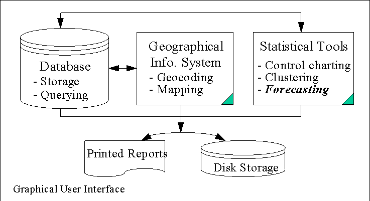
This work supports the addition of a forecasting or prediction component to the Regional Crime Analysis Program (ReCAP) developed at the University of to support crime analysis in the Abemarle County, Charlottesville City, University of Virginia, and Richmond Police departments. The ReCAP system is an interactive shared information and decision support system that includes these components - a database, geographical information system (GIS), and statistical tools (Brown, 1998). The fully functional system consists of the seamless integration of all the components (Figure 1).

Figure 1. ReCAP Components

Our goal in forecasting is to develop the likelihood or density that another crime incident occurs at some location within a monitoring region. This region is defined by police jurisdictions. To conduct this forecasting we will employ any retrievable information in the database about the past incidents of the same type, i.e., their locations and times of occurrence, and any relevant crime scene characteristics or features. The resulting predicted likelihoods or probability density function for criminal events can be mapped out by the GIS. The resulting map is obviously useful for making decisions on allocation of police resources and reducing response time to problem areas.

Effective and efficient prediction also involves identifying key characteristics or features as a preliminary step. The key features, if identified, can be considered the common threads behind the crime incidents of the same type, and thus provides useful information to understand the nature of the type of crime under investigation.

The practical significance of this work in support of tactical decision making in law enforcement is obvious: the better we forecast criminal activity then the better we can allocate law enforcement resources to combat it. However, the usefulness and significance of these forecasting models goes beyond tactical decision making. In the emerging field of computer-based crime analysis and law enforcement support, the existing software has concentrated on static analysis of aggregate data. This analysis tends to encourage reactive rather than proactive planning and resource allocation. Predictive models provide a way to address criminal activity proactively and, therefore, more effectively support community policing, problem-oriented policing, and cooperation among agencies.

The remainder of this paper consists of sections that describe related work (Section 2), our model for predicting criminal events without the mathematical details (Section 3), results from applying to model to predicting events in the Richmond area (Section 4), and conclusions (Section 5).

This section reviews related work for predicting spatial-temporal events. We start with general methods, examine the theories on the spatial component of crime, and then look at some recent applications to law enforcement.

2.1 Stochastic Point Processes

General methods for forecasting events in space and time derive from the area of stochastic point processes. In this area initial work attempted to generalize results from time series analysis. However, spatial processes are not unidirectional as are temporal processes. Hence, additional work attempted to build a theory of spatial point processes. The basic concepts and characterization of point patterns in time can be found in standard stochastic modeling texts such as Karlin and Taylor (1975) and Taylor and Karlin (1984), and texts devoted to time series modeling, e.g., Cox and Lewis (1966), Lewis (1972), and Snyder (1975). Early studies of spatial point patterns were primarily concerned with comparing area (or quadrat) counts to a Poisson distribution (e.g., Student, 1907); tests indicate departures from the null hypothesis of Complete Spatial Randomness (CSR) (e.g., Neyman, 1939). Many of the early results have been developed outside statistics and can be collectively viewed as exploratory or descriptive tools measuring the degree of departure from CSR. These include quadrat counts (e.g., Fisher et al., 1922; David and Moore, 1954; Morisita, 1959; Lloyd, 1967), distance measures between events, points, and other things (e.g., Skellam, 1952; Clark and Evans, 1954; Hopkins, 1954), and the K function (e.g., Ripley, 198e). The development of formal models for spatial point patterns owes much to the work of Matthes et al. (1978), Kellenberg (1986), Karr (1986), and Daley and Vere-Jones (1988). A major focus in space-time patterns has been the development of methods for testing space-time clustering (e.g., Knox, 1964; Ederer et al., 1966; Mantel 1967; Pike and Smith, 1974; McAuliffe and Afifi, 1984; and Chen et al., 1984). A lack of a theory of space-time point pattern is frequently identified in the literature, and the majority of the models were developed for specific applications (e.g. mining or hydrology). Fiksel (1984) proposed some space-time cluster models for a sequence of geological events with the assumption that they are from a Markov process. In the water resources literature, the work by Smith and Karr (1983, 1985a, 1985b), Jacobs et al. (1988), Rodriguez-Iturbe et al. (1988) model rainfall events and the evolution of rain cells.

In the area of "space-time prediction" the use of "kriging" is frequently cited. This term actually applies to interpolating a continuous measurement over a region based on its observed values at various known locations (see, for example, Matheron, 1963). Other space-time models have extended time series methods to the spatial domain. Among the research in this area the development of space-time autoregressive-moving-average (STARMA) models (Cliff et al., 1975) has been particularly important. STARMA models offer a way of generalizing both the autoregressive-moving-average (ARMA) time-series models and the simultaneously specified spatial models. These models are characterized by linear dependence lagged in both space and time. Several authors (Martin and Oeppen, 1975; Aroian, 1980; Pfeifer and Deutsch, 1980a; and Abraham, 1983) discussed issues of stationarity and invertibility arising from model parameter estimation. Unfortunately, these studies were based on an unrealistic assumption that spatial dependence is instantaneous. The STARMA model was further generalized by Pfeifer and Deutsch (1980b) to include temporal differences (STARIMA models) and by Stoffer (1985, 1986) to include a nonstationary mean function of independent variables (STARMAX models). They also argue that spatial processes lack homogeneity and this must be reflected in spatial models. In particular, most existing methods do not take advantage of the extra incident-related feature information which is more localized. For instance, crimes that occur at specific locations have demographic and distance relationships to other features (e.g. schools and churches). Hence, spatial variables are local and should be modeled based on each incident type. Our proposed predictive models will use this added information.

Another approach to space-time modeling has been to apply neural networks. Neural networks encompass a wide variety of techniques. However, the most commonly used of these techniques are multi-layer perceptrons or back-propagation neural networks. Olligchlaeger (1997) has recently studied the use of back-propagation neural networks and cellular automata for forecasting 911 calls. His results were comparable to those of multiple regression. While neural networks have shown excellent accuracy in many applications, they have some disadvantages for criminal event predictive modeling, because they are black boxes. This means that the user gains no process insight from these models and, hence, their usefulness for community policing and problem-oriented policing as described in Section 1 is limited.

2.2 Spatial Theories of Criminal Activity

The spatial component of crime has been well documented and hence, the application of crime analytic techniques to understanding this component has also been significant. This subsection makes no claim to completeness in the discussion of this rich source of work. Instead our intent here is to provide a brief summary of this literature as a motivation to our work in predictive modeling.

One of the most complete discussions of spatial patterning in crime is contained in (Brantingham and Brantingham 1984). From the standpoint of this paper we are particularly interested in what they call the microspatial component of crime or the choice of criminal locations by individual criminals. A number of researchers have documented and formulated descriptions for spatial decision making by criminals (see, for example, Brantingham and Brantingham 1975, Molumby 1976, Newman 1972, Repetto 1974, Scarr 1973). Some have looked specifically at the question of distance from home to crime location (for example, Amir 1971, Baldwin and Bottoms 1976, Capone and Nichols 1976, LeBeau 1987, Rossmo 1993, Rossmo 1994). Taken together this impressive body of research shows that "target selection is a spatial information processing phenomenon." (Brantingham and Brantingham 1984, p. 344). Essentially offenders use spatial attributes in their site selection. We will use this concept in Section 3 to describe our models for predicting criminal activity. There we will refer to these spatial attributes as features or attributes that define the preference of offenders for specific sites.

The evident spatial element of criminal behavior has meant that law enforcement personnel have for centuries included spatial analysis in their work. Weisburd and McEwen (1997a) provide a brief history of crime mapping in law enforcement going back to the early 1800s. The advent of GIS has made possible new types of spatial analysis of crime and created an explosion of interest in crime mapping (see, e.g. Block and Dabdoud 1993, Block, Dabdoud, and Fregly 1995, Harries 1990, Weisburd and McEwen 1997b,). This work suggests that we now have in place the mapping tools (GIS), the database tools, and some analytical methodology. However, most law enforcement agencies are using these tools as obvious computer-based versions of the old pin-mapping techniques. The combination of computer hardware and software provides us the opportunity to do considerably more with the data available. Not surprisingly many people have identified this need and built tools to address various aspects of it. We briefly examine some representative tools in the next section.

2.3 Law Enforcement Tools

A variety of tools have been developed to aid law enforcement in performing crime analysis and some of these specifically focus on spatial analysis. However, none of them provide predictive modeling capabilities as we describe here. We begin this short review with more general crime analysis systems and then look specifically at spatial crime analysis systems.

Examples of general crime analysis support systems include the Armed Robbery Eidetic Suspect Typing (AREST) (Badiru, et al. 1988), VICAP (Icove 1986), Big Floyd (Gilman 1987), APES (Coady 1987) and the Baltimore County Burglary System (Ratledge and Jacoby1989). None of these systems explicitly use spatial analysis or predictive modeling.

All of the above systems were based on expert systems ideas. Statistical methods have also been exploited for crime analysis support systems. An early example of a statistical model-based approach is in Harris (1978). More recently Gottlieb, et al. (1994) have codified this approach. They show how to employ simple statistical models to describe the behavior of criminals in an area. This idea combined with information processing techniques has been implemented in a wide variety of software products, such as Watson (Security Management 1994), Memex, iGlass, ALTAanalytics, and SIUSS. All of these products find links between data elements but they do not provide predictive modeling or spatial analysis.

In addition to general crime analysis systems, a number of researchers, law enforcement agencies, and commercial companies have built spatial analysis support systems. Geake (1993) describes the Crime Pattern Analysis System, which looks at spatial displays and summary statistics. The San Bernadino County Sheriff�s Department (Miller, 1994) developed a program with similar capabilities. The San Diego police have also employed GIS to help understand crime patterns in their area (Newcomb, 1993). STAC, which was developed by Carolyn Block (Block, 1995), is a good example of a well-developed spatial analysis tool. However, none of these systems provide predictive modeling capabilities.

Many other spatial tools are listed in the books edited by Block, Dabdoud, and Fregly (1995) and Weisburd and McEwen (1997b). The only predictive approach described in these references is the work by Olligschlaeger described in Section 2.1. Again, this effort provided good predictive results for calls for service, but because it used a neural network approach it lacks explanatory power as needed for community policing and problem-oriented policing, in particular.

3. Predictive Model Using Offender Preference Discovery

The basic idea behind our approach derives from the theories of criminal activity summarized in Section 2.2. Offenders choose the place and time to offend based on a set of attributes that describe that place. These attributes can include the presence or absence of police, the distance to the nearest major highway for quick exits, the presence of home with valuables, etc. We would like to know both the attributes and trade-offs among the attributes used by the offender. Trade-offs are important because offenders (like everyone else) cannot get exactly what they want on all attributes. For example, an offender may choose a more distant home to rob because it possesses a less sophisticated security system, thus valuing the reduced risk of apprehension more highly than convenience to the site.

If we knew the attributes used by the offenders and their trade-offs among these attributes then we could evaluate all potential sites and score them accordingly. Obviously, we do not have this information. So we need an approach to the discovery of these offender preferences. But first we need a way to model the information in the environment and mechanism for describing change in the environment.

Figure 2 shows a symbolic view of our modeling approach. We the geographic space in which the offenders act in terms of a grid. Each grid point contains attributes that describe the state of the environment at that grid point. For example, the state information for a single grid point might contain the number of bars, family density, and number of robberies and other facts pertinent to that grid point.

Figure 2 also shows that the information at the grids change from one time to the next. This is obvious for facts like the number of robberies which will change from one day, week or month to the next. However, we generally do not know the mechanism for this process. If we can discover the offender preferences then we can provide the mechanism we need to predict changes from one time to the next.

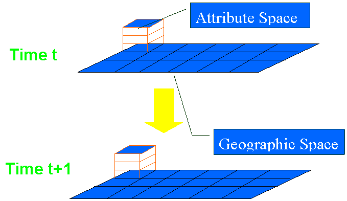
Figure 2. State Space Modeling Approach

Figure 3 provides a schematic of our approach to the discovery process. At the top of the figure is the temporal axis. This shows the times when the criminal incidents occur. At the bottom of the diagram are the spatial dimensions showing the locations of the crime. In the middle we depict the feature or attribute space. These dimensions show the values of the criminal incidents on each of the many possible attributes used by the offender.

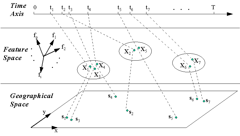
Figure 3. Schematic Representation of the Model for Preference Discovery

If the offenders behave consistently in their choices among these attributes then the incidents will tend to cluster. As we noted in Section 2.2, the theories of criminal behavior the choice of site is a spatial information processing task. The values of the features at a site make it either attractive or unattractive to offenders. The clusters in feature space reveal the regions of attraction.

Our approach first finds these clusters in feature space. We employ several methods to perform the clustering and the details can be found in (Liu and Brown, 1998) and (Liu, 1999). Essentially these methods do more than cluster. They actually provide a probability model in feature space. This model has the following characteristic: regions near to high density groupings in feature space have a greater likelihood of being chosen for future criminal incidents than regions far from high density areas.

But the question remains as to the choice of the attributes to use. Since we want to find the attributes or features relevant to offenders' choices, we start with a large set of possible features. This gives us some confidence but obviously not assurance that we will subsume the set of features used by the offenders. However, the price we pay for this approach is computational complexity. A large number of attributes means a search (unfortunately, an intractable search) for the ones that offenders use.

Ideally we hope to recover the offenders' attribute set from the initial attribute set. However, we can never know (even with post arrest interviews) if we have chosen correctly. So our goal is somewhat more modest: we want the smallest set of attributes that produces the observed spatial-temporal pattern. The resulting attribute set will also be useful in helping to understand criminal processes.

Our approach to attribute or feature selection is given in more detail in (Brown and Liu, 1998 and Liu 1999). In this paper we provide an intuitive description of the approach. Suppose that perform our clustering in feature or attribute space and find K clusters (again, our approach actually does not produce distinct clusters, but this simplification is useful for purposes of explanation). Now if we knew the offenders' attributes and did the same clustering using just these attributes we would find C clusters. We claim that K � C because as we add more superfluous dimensions, clusters can split but not combine. So in our approach we conduct a search using the following objectives:: (1) maximization of the average tightness of the clusters in the reduced feature space defined by the selected subset of features; (2) minimization of the number of features used; and (3) minimization of the departure from the mapping property that we should have observed if the feature subset being examined were the offenders' feature set.

4. Example Application

We applied the approach described in the previous Section to data from Richmond, Virginia. The data consist of 579 forcible breaking and enterings that occurred between July 1, 1997 and August 31, 1997. We looked at weekly aggregations of these data. We considered 100 features as the potential basis for offender preferences. These included census data such as income, population densities, and distances to landmarks (schools, government buildings, roads, etc.).

We note that many of these features are very coarse. In particular, the census data were available to only the block group level, while our grids were 2624.84 meters on a side.

We used data from July 7, 1997 to July 21, 1997 to train or serve as the basis for building the model. These two weeks of data then served for feature selection and for prediction for the next weeks.

When we applied our feature selection algorithm to these two weeks of data it chose three features: family density by block group; personal care expenditures per family per block group; and distance to the nearest highway. Again, coarseness of the features available undoubtedly was the basis for this selection of features. Figure 4 shows the family density feature and with the actual crimes in the data set.

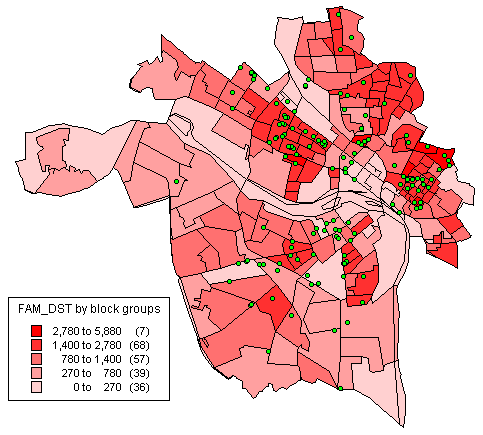
Figure 4. Family Density Feature, Richmond, Va.

Even with these three coarse features we obtained good results for predicting one and two weeks ahead. Figure 5 shows the prediction for one week in advance and figure 6 shows the two week prediction. The intensity of the gray scale shows the likelihood of a criminal event and the dots show the actual locations for the events. We obtained these results using a mixture model approach to density estimation.

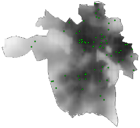
Figure 5. One Week Prediction Surface, Richmond, Va.

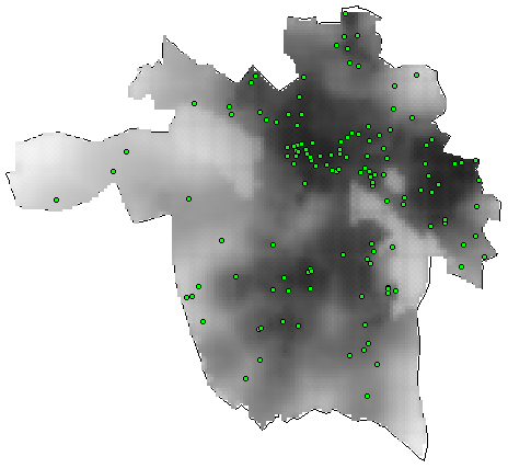
Figure 6. Two Week Prediction Surface, Richmond, Virgina.

In addition to comparing the prediction surface to actual incidents as shown in Figures 5 and 6, we also conducted formal tests of prediction accuracy. To do this we used a base case prediction model obtained by clustering (or more precisely, constructing density estimates of) the 2 weeks of training data. This clustering or estimation used only the locations of the crimes. This technique essentially finds hot spots of criminal activity and then predicts future crimes based on existing crimes.

To compare our preference discovery approach with these hot spot approach we used percentile scores. A percentile score computes the percentile of each actual crime point in the probability surface generated by each method. So, for example, if a point occurs near the maximum of a probability surface it gets a percentile score close to one. Points near the minima of the prediction surface get percentile scores close to zero. If our approach does better than the hot spot techniques then it should have higher percentile scores for each crime point that occurs during the two week period that we try to predict.

In fact in all tests that we ran the preference discover approach provides higher average percentile scores than the hot spot method and this difference is statistically significant (at the 0.1) in all but one case. This provides strong evidence that the approach is performing well in predicting these data.

5. Conclusions

One of the more important contemporary questions for crime analysts and criminologists concerns the predictability of criminal events. The tools are now available in many jurisdictions to enable new approaches to this problem. This paper has described an approach that uses current criminology theory and data available through GIS. Specifically the approach discovers and models offender behavior to predict locations of future criminal events. It also finds those features useful for prediction

Testing of this approach shows that even with coarse features it can predict criminal events with greater accuracy that hot spot analysis. This suggests that criminal behavior can be predicted from spatial and attribute data.

Author Affiliation

Acknowledgements

This work was partially supported by grants from the Crime Mapping Research Center, National Institute of Justice and from the Virginia Department of Criminal Justice Services.

References

Abraham, B. (1983). The exact likelihood function for a space-time model. Metrika, 30, 239-243.

Amir, M. (1971) Patterns in Forcible Rape, University of Chicago Press, Chicago.

Aroian, L. A. (1980). Time Series in m dimensions: Definitions, problems, and prospects. Communications in Statistics, Simulation and Computation, B9, 453-465.

Badiru, A. B., J. M. Karasz, and R. T. Holloway. (1988) AREST: Armed Robbery Eidetic Suspect Typing Expert System. Journal of Police Science and Administration. 16:210-216.

Baldwin, J. and Bottoms, A. (1976) The Urban Criminal: A Study in Sheffield, Tavistock Publications, London.

Block C.R. and Dabdoud, M. (1993) Workshop on Crime Analysis Through Computer Mapping Proceedings, Illinois Criminal Justice Information Authority, Chicago.

Block, C. (1995) STAC Hot-Spot Areas: A statistical tool for law enforcement decisions, in Crime Analysis Through Computer Mapping, ed. by C. R. Block, M. Dabdoub, and S. Fregly, Police Executive Research Forum, Washington, D.C., 20036.

Block C.R., Dabdoud,M., and Fregly, S. (1995), editors, Crime Analysis Through Computer Mapping, Police Executive Research Forum, Washington, D.C., 20036

Brantingham, P. and P. Brantingham (1975), Spatial Patterns of Burglary, Howard Journal of Penology and Crime Prevention, 14, 11-24.

Brantingham, P. and P. Brantingham (1984) Patterns in Crime, Macmillan Publishing Company, New York.

Brown, D. E.(1998) "Data Mining to Catch Criminals: The Regional Crime Analysis System (ReCAP)" Proceedings of the IEEE International Conference on Systems, Man, and Cybernetics, October 1998, San Diego, California.

Capone, D. and Nichols, W. (1976) Urban Structure and Criminal Mobility, American Behavioral Scientist, 20, 199-213.

Chen, R., Mantel, N., and Klingberg, M. A. (1984). A study of three techniques for space-time clustering in Hodgkin�s desease. Statistics in Medicine, 3, 173-184.

Clark, P. J. and Evans, F. C. (1954). Distance to nearest neighbor as a measure of spatial relationships in populations. Ecology, 35, 445-453.

Cliff, A. D., Hagget, P., Ord, J. K., Bassett, K. A., and Davies, R. B. (1975). Elements of Spatial Stucture: A Quantitative Approach. Cambridge University Press, Cambridge.

Coady, W. F. (1987) "Investigating with APES." Security Management. 31:67-70.

Cox, D. R. and Lewis, P. A. W. (1966). The Statistical Analysis of Series of Events. Methuen, London.

David, F. N. and Moore, P. G. (1954). Notes on contagious distributions in plant populations. Annals of Botany, 18, 47-53.

Daley, D. J. and Vere-Jones, D. (1988). Introduction to the Theory of Point Processes. Springer, New York.

Ederer, F., Myers, M. H., and Mantel, N. (1966). A statistical problem in space and time: Do leukemia cases come in clusters? Biometrics, 20, 626-638.

Fiksel, T. (1984). Simple spatial-temporal models for sequences of geological events. Elektronische Informationsverarbeitung und Kybernetik, 20, 480-487.

Fisher, R. A., Thornton, H. G., and Mackenzie, W. A. (1922). The accuracy of the plating method of estimating the density of bacterial population. Annuls of Applied Biology, 9, 325-359.

Geake, E. (1993), How PCs predict where crimes will strike, New Scientist, Oct. 23, 1993, p. 17.

Gilman, H. (1987) "Detectives on disks: Law enforcers use new computer software to solve crimes," Wall Street Journal, p. 29, September 11.

Gottlieb, S., S. Arenberg, and R. Singh (1994) Crime Analysis from First Report to Final Arrest, Alpha Publishing.

Harries, K.D. (1990) Geographic Factors in Policing, McGraw-Hill, New York, NY.

Harris, D. H. (1978) "Development of a Computer-Based Program for Criminal Intelligence Analysis" Human Factors. 20 (February), 47-56.

Hopkins, B. (1954). A new method for determining the type of distribution of plant individuals. Annuals of Botany, 18, 213- 227.

Icove, D. J. (1986) Automated Crime Profiling. Law Enforcement Bulletin. 55:27-30.

Jacobs, B. L., Rodriguez-Iturbe, I., and Eagleson, P. S. (1988). Evaluation of a homogeneous point process description of Arizona thunderstorm rainfall. Water Resources Research, 24, 1174-1186.

Karlin, S. and Taylor, H. (1975). A First Course in Stochastic Processes. Academic Press, New York.

Karr, A. F. (1986). Point Processes and their Statistical Inference. Marcel Dekker, New York.

Kellenberg, O. (1986). Random Measures, 4th ed. Academic Press, New York.

Knox, E. G. (1964). The detection of space-time interactions. Applied Statistics, 13, 25-29.

LeBeau, J.L. (1987) The Journey to Rape: Geographic Distance and the Rapist�s Methods of Approaching the Victim, Journal of Police Science and Administration, 15, 129-136.

Lewis, P. A. W. ed. (1972). Stochastic Point Processes: Statistical Analysis, Theory, and Applications. Wiley, New York.

Liu, H. "Space-Time Point Process Modeling: Feature Selection and Transition Density Estimation." Ph.D. Dissertation, University of Virginia. May 1999.

Liu,H. and D.E. Brown (1998) "Spatial-Temporal Event Prediction: A New Model," Proceedings of the IEEE International Conference on Systems, Man, and Cybernetics, October 1998, San Diego, California.

Lloyd, M. (1967). Mean crowding. Journal of Animal Ecology, 36, 1-30.

Mantel, N. (1967). The detection of disease clustering and a generalized regression approach. Cancer Research, 27, 209-220.

Martin, R. J. and Oeppen, J. E. (1975). The identification of regional forecasting models using space-time correlation functions. Transactions of the Institute of British Geographers, 66, 95-118.

Matheron, G. (1963). Principles of geostatistics. Economic Geology, 58, 1246-1266.

Matthes, K., Kerstan, J. and Meche, J. (1978). Infinitely Divisible Point Processes. Wiley, New York.

McAuliffe, L. and Afifi, A. A. (1984). Comparison of a nearest-neighbor and other approaches to the detection of space-time clustering. Computational Statistics and Data Analysis, 2, 125-142.

Miller, T. (1994) Computers track the criminal trail, American Demographics, January, pp. 13-14.

Molumby, T. (1976) "Patterns of Crime in a University Housing Project," American Behavioral Scientist, 20, 247-259.

Morisita, M. (1959). Measuring of the dispersion and analysis of distribution patterns. Memoires of the Faculty of Science, Kyushu University, Series E. Biology, 2, 215-235.

Newcomb, T. (1993) "High tech tools for the war on crime," Governing, August, pp. 20-21.

Newman, O. (1972) Defensible Space: Crime Prevention Through Urban Design, Macmillan, New York.

Neyman, J. (1939). On a new class of "contagious" distributions, applicable in entomology and bacteriology. Annals of Mathematical Statistics, 10, 35-37.

Olligschaeger, O. (1997) Artificial neural networks and crime mapping, in Crime Mapping and Crime Prevention, ed.by D. Weisburd and T. McEwen, Criminal Justice Press, Money, NY.

Pike, M. C. and Smith, P. G. (1974). A case-control approach to examine diseases for evidence of contagion, including diseases with long latent periods. Biometrics, 30, 263-279.

Pfeifer, P. E. and Deutsch, S. J. (1980a). Indentification and interpretation of first order space-time ARMA models. Technometrics, 22, 397-408.

Pfeifer, P. E. and Deutsch, S. J. (1980b). A three-stage iterative procedure for space-time modelling. Technometrics, 22, 35-47.

Ratledge, E. C. and J. E. Jacoby. Handbook on Artificial Intelligence and Expert Systems in Law Enforcement. New York: Greenwood Press, 1989.

Repetto, T.A. (1974) Residential Crime, Ballinger, Cambridge, MA.

Ripley, B. D. (1981). Spatial Statistics. Wiley, New York.

Rodriguez-Iturbe, I. and Eagleson, P. S. (1987). Mathematical models of rainstorm events in space and time. Water Resources Research, 23, 181-190.

Rosmo, D.K. (1993) "Target Patterns of Serial Murders: A Methodological Model," American Journal of Criminal Justice, 17(2), 1-21.

Rosmo, D.K. (1994) "Targeting Victims: Serial Killers and the Urban Environment," in Serial and Mass Murder: Theory, Research, and Policy, ed. by T.O�Reilly-Flemming and S. Egger, University of Toronto Press, Toronto.

Scarr, H.A. (1973) Patterns in Burglary, 2^nd Ed., U.S. Dept. of Justice, Washington, D.C.

Security Management (1994) "Software Solution," 38 (March), 17.

Skellam, J. G. (1952). Studies in statistical ecology, I: Spatial pattern. Biometrica, 39, 346-362.

Smith, J. A. and Karr, A. F. (1983). A point process model of summer season rainfall occurrences. Water Resources Research, 19, 95-103.

Smith, J. A. and Karr, A. F. (1985a). Statistical inference for point process models of rainfall. Water Resources Research, 21, 73-79.

Smith, J. A. and Karr, A. F. (1985b). Parameter estimation of a model of space-time rainfall. Water Resources Research, 21, 1251-1257.

Snyder, D. L. (1975). Random Point Processes. Wiley, New York.

Stoffer, D. S. (1985). Maximum likelihood fitting of STARMAX models to incomplete space-time series data. In Time Series Analysis: Theory and Practice 6, O. D. Anderson, J. K. Ord, and E. A. robinson, eds. North-Holland, Amsterdam, 283-296.

Stoffer, D. S. (1986). Estimation and identification of space-time ARMAX model s in the presence of missing data. Journal of the American Statistical Association, 81, 762-772.

Student (1907). On the error of counting with a haemacytometer. Biometrika, 5, 351-360.

Taylor, H. and Karlin, S. (1984). An Introduction to Stochastic Modeling. Academic Press, New York.

Weisburd, D. and McEwen, T. (1997a) "Introduction: Crime Mapping and Crime Prevention," in Crime Mapping and Crime Prevention, ed. by D. Weisburd and T. McEwen, Criminal Justice Press, Monsey, NY.

Weisburd, D. and McEwen, T. (1997b), editors, Crime Mapping and Crime Prevention, Criminal Justice Press, Monsey, NY.