Screening-Level GIS Tools for Modeling Environmental Contamination from Mining Activities

Ferdi Hellweger, Eugenia Naranjo, Pete Shanahan, Ken Fellows, Gary Ostroff and Paul Anid

ABSTRACT

A geographic information system (GIS) was developed to support the management of existing and future mining activities in Bolivia. Basic GIS functionality (e.g. zooming and layering) is provided by Esri�s ArcView GIS software and supplement by three screening-level environmental modeling tools. These tools estimate the impact of mining activities on surface water, groundwater and air quality in and around mining centers across Bolivia.

The models compute steady-state metal exposure concentrations in surface water, groundwater and the air. The model results are presented as new data layers (themes) in the GIS, allowing exposure concentration to be overlaid onto population centers. The output of the surface water model is represented as colored (or thickened) lines, and X/Y plots of concentration vs. distance can also be created. The output of the groundwater and air models is presented as contours of metal concentrations.

The models are fully integrated with the graphical user interface (GUI) of ArcView. The user interacts with the models through pop-up windows. The input and output of the models is stored in the GIS database. All the models are in FORTRAN code that is executed off-line. The models are run this way, because processing speed is an important factor for numerical modeling and FORTRAN is much faster than Avenue. The surface water model, for example, uses EPA�s WASTOX framework.

The focus of this paper is on the integration of the models with the GIS.

INTRODUCTION

Bolivia has a rich mining history, which began in the mid-1500s when silver was discovered in the town of Potosi. The wealth generated by this strike underwrote the Spanish economy for over two centuries. Since then, the importance of mining in Bolivia has declined, but gold, zinc, tin and silver are still mined in significant quantities. Collectively, the mining industry still accounts for about 50% of the country�s exports.

Past and present mining activities in Bolivia cause considerable environmental damage to the air, surface water and groundwater. Smokestacks from smelter facilities emit metal and other contaminants. Waste rock piles (tailings) and mine discharges cause acidification and metal contamination of surface water and groundwater.

Presently, the Bolivian mining sector is undergoing major restructuring. The state mining corporation of Bolivia (COMIBOL) has introduced several changes and closed a number of mines. Mines with the potential of being profitable are being offered for private participation. As part of this process, COMIBOL, the Vice-Ministry of Mining and Metallurgy (VMMM) and the Bolivian Geological survey (SERGEOMIN) are addressing the environmental damage caused by present and future mining activities. An Environmental Information System (EIS) was developed to provide the Bolivian government with a screening-level management tool.

ENVIRONMENTAL INFORMATION SYSTEM

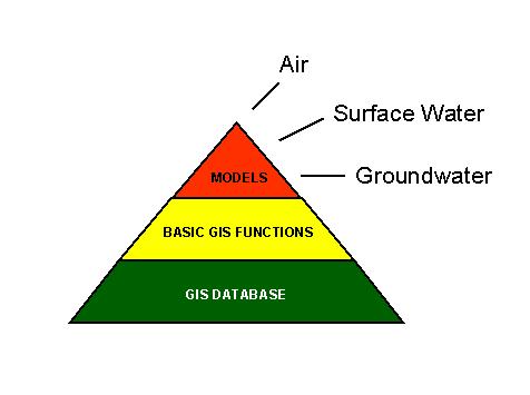
The tool developed is termed an Environmental Information System (EIS). A conceptual view of this EIS is presented in Figure 1. Its foundation is a geographic information system (GIS) database supplemented with basic GIS functionality provided by Esri�s ArcView GIS software. Also, three models are constructed to supplement the basic GIS functionality. Those models predict concentrations of metals in air, surface water and groundwater.

Figure 1. Environmental Information System (EIS).

The sections below provide a brief description of the models used as well as references to more detailed information.

Surface Water Model

The surface water model uses the WASTOX code, which is a toxic chemical fate and transport model developed by Manhattan College and the US Environmental Protection Agency (US EPA) and now supported by the US EPA. The following paragraph is from the WASTOX documentation (Connolly and Winfield, 1980):

The program permits the user to model the water and sediment transport in a natural water system and the movement and decay of a chemical continually discharged to the system or the concentration in the system as a function of time may be computed. The reaction of the chemical and its transfer between phases are computed from specified characteristics of the chemical and environmental parameters of the system.

Air Model

The air model uses the Industrial Source Complex � Short term, Version 3 (ISCST3) code developed and maintained by the US EPA (1995). ISCST3 is a widely used and tested atmospheric dispersion model, which predicts annual average ground level pollutant concentrations. The model is a Gaussian plume model that considers the pollutant concentration in the plume to be normally distributed in both the horizontal and vertical directions. Dispersion of the plume as it moves downwind occurs as a result of atmospheric turbulence.

The technique used for predicting contaminant transport in ground water is that described by Wilson and Miller (1978, 1979) for a continuous mass source in horizontal, two-dimensional, uniform ground-water flow. The solution assumes that the contaminants are in dissolved form and are subject to linear decay and linear equilibrium sorption. The solution is an exact analytical representation of the concentration distribution downgradient of a line source, introduced uniformly over the vertical thickness of an aquifer. It may also be used with reasonable accuracy, as in the present case, for situations where only the far field concentration is of interest.

The GIS/Model integration methodology is presented in Figure 2. The left part of the Figure illustrates the conceptual view of a GIS where the user interacts with a database through software. In this case, Esri�s ArcView GIS software was selected, because it is powerful and easy to use. ArcView provides the basic GIS functionality including editing features, zooming and identifying features (ID).

The right part of the Figure illustrates the traditional conceptual view of the environmental modeling process. Models are usually pictured as black boxes that take input and compute output. This concept does not agree well with that of the GIS and integration of the two concepts is challenging. There are several possible options for integrating the model with the GIS. We chose to keep the modeling process (input-model-output) intact and separate from the GIS (models are run off-line). This allowed us to use published, tested models, without the need for extensive code development.

To integrate the model with the GIS we wrote a set of programs in ArcView�s Avenue programming language. The programs manage the complete modeling process: They write the input, execute the model and read the output. From the user�s perspective, both model input and output are stored in the GIS database. The input file read by the model code and the output file generated by the model are considered temporary communication devices.

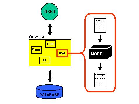
Figure 2. GIS/Model Interface Methodology.

As mentioned above, the model input and output are stored in the GIS database of the EIS as illustrated in Figure 3. The input consists of spatial and constant parameters (the models are steady state so there are no time variable parameters). Spatial information is stored in ArcView Shape Files and ARC/INFO Grids, while constant information is stored in dBASE tables. The output of the models is spatially varying metal concentrations, so that information is stored in Shape Files and Grids as well.

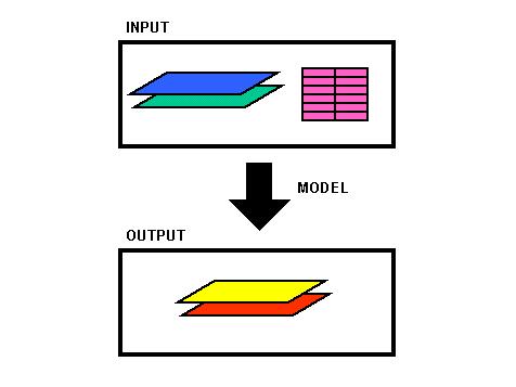
Figure 3. Model Input/Output Data Types.

The user interface of the models is embedded in ArcView�s graphical user interface (GUI). Since it is similar for all three models only the one for the surface water model will be presented here as illustrated in Figure 4. The buttons used to access the model are color coded so that they can be distinguished from the standard ArcView buttons.

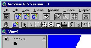
Figure 4. Surface Water Model User Interface (M, C, G and E buttons).

The functionality of the buttons is as follows:

M � Execute Model
C � Edit Constant Parameters
G � Graph Results
E � Edit Spatial Parameters

Spatial information is stored in Shape File attribute tables. They are viewed and/or edited using the E tool. Clicking on a feature will cause a dialog box to be displayed. Figure 5 shows the dialog box used to view/edit the reach parameters for the surface water model. Once the user has entered the information the attribute values of that particular stack are updated.

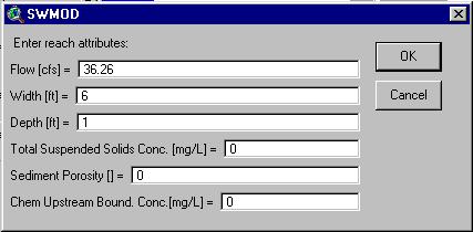
Figure 5. Surface Water Model Reach Parameter Edit Dialog Box.

Constant parameters are edited using the C button. Figure 6 illustrates the dialog box for the surface water model. The constant parameter values are stored in a dBASE table.

Figure 6. Surface Water Model Constant Parameter Edit Dialog Box.

In a typical application of the model the user focuses on an area of limited geographic extend and model calculations would to be restricted to that area. A procedure for limiting the model extent was therefore set up. In general, the user selects the features to be included in the model using ArcView's generic �select feature� tool. Figure 7 shows an example where the user has selected four sources and a number of river reaches to be included in the model.

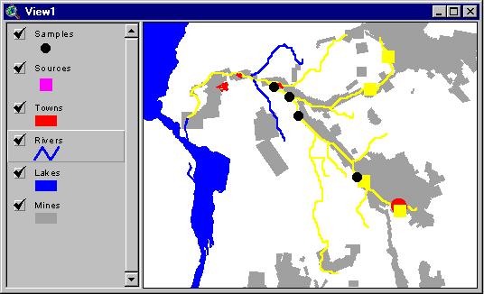
Figure 7. Surface Water Model Feature Selection.

This type of model user interface is tightly integrated with the geographic information and thus can be termed a geographic user interface or GeoUI.

The model is executed using the M button. The user is prompted for a run name, which will be used to name the output of the model. The system will also save the input information under the same name. This is done, because the input data layers (e.g. rivers and sources) are dynamic and change with time. Figure 8 shows the dialog box for the surface water model.

Figure 8. Surface Water Model Run Name Dialog Box.

The model is executed in an MS DOS window as illustrated in Figure 9. Once the model is finished the MS DOS window is automatically closed.

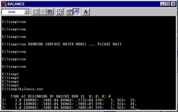
Figure 9. Surface Water Model Execution in MS DOS Window.

The output of the models is presented as a new layer (theme) in the View, named using the run name specified by the user. A coloring scheme (classification) is applied automatically based on the range of output concentrations. Figure 10 shows the output of a surface water model simulation. Note that the model only computed concentrations for the features selected (see Figure 7).

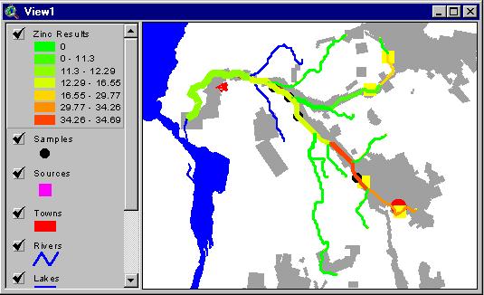
Figure 10. Surface Water Model Results for Zinc [mg/L].

In this case Zinc was modeled. Note that the general pattern of the model output is correct. Concentrations are highest directly downstream of the sources and then decline due to dilution. The model predicts concentrations up to about 35 mg/L, which is higher than the 3 mg/L World Health Organization (WHO) standard for drinking water.

Another feature of the surface water model is the G button. This is a tool to plot concentrations along the river. Figure 11 shows the modeled Zinc concentrations along the main stem of the river.

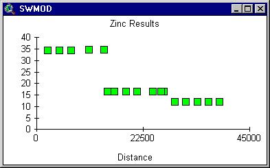
Figure 11. Surface Water Model XY Plot for Zing [mg/L]

The output of the air model is mean annual exposure concentrations of metals at ground level. Figure 12 shows the results of a Lead simulation.

Figure 12. Air Model Results for Lead [ug/m3].

In general the concentrations are highest on the north side of the stacks, because the prevailing wind direction in that area is from the southeast. Also note that the highest concentrations are not directly at the stacks, because the output concentrations are at ground level and it takes some distance for the plume to wash down to ground level. The highest contour corresponds to a concentration of 0.01 ug/m3. This can be compared to the US EPA criteria value for human health, which is 1.5 ug/m3. There is a slight inconsistency in that the modeled concentration is an annual mean and US EPA criteria value is for a quarterly average. Nevertheless the comparison demonstrates that the lead emissions from this group of stacks does not pose a risk to human health. Figure 13 shows the results for arsenic.

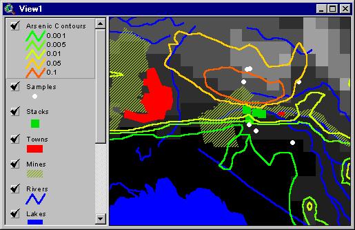
Figure 13. Air Model Results for Arsenic [ug/m3].

The US EPA criteria value for human health for arsenic is 0.05 ug/m3, which corresponds to the second highest contour line in the Figure. The overlay capabilities of ArcView allow for the contours to be viewed in direct relation to the population centers.

Once the model has created the output layers the user can manage them using standard ArcView functions. This includes, for example, applying a different coloring scheme (classification) to the layers using ArcView�s legend editor. Figure 14 shows how the results of two different groundwater model simulations are compared.

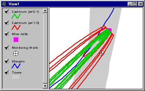
Figure 14. Comparison of Two Separate Groundwater Model Results.

The model results are for Cadmium concentration. In this case there was considerable uncertainty about the transverse dispersivity property (dispersion) of the aquifer. The model was therefore run several times with different dispersivities to estimate the range of likely output concentrations. Figure 14 shows the model results with the dispersivity set to the lower (0.1 m, green lines) and higher (1.0 m, red lines) end of the likely range.

Three screening level models were developed that compute steady-state exposure concentration of metals in air, surface water and groundwater. The user interacts with the models through the ArcView user interface, which provides the models with a geographic user interface (GeoUI).

Executing environmental models off-line allows for the use of established and tested modeling codes. This adds credibility to the models and reduces the amount of coding to be done. Another reason for running models �off-line� is the significantly higher execution speed of FORTRAN over Avenue.

Storing model input and output in the GIS database was found to be very beneficial. This way the user can use the data management functions of ArcView to edit and view the information. Model results can be colored using ArcView�s legend editor and overlaid with other layers (e.g. population centers).

Funds for this project were provided by a World Bank Credit #Aif-2805-BO to the Corporacion Minera de Bolivia (COMIBOL) and Viceministerio de Mineria y Metalurgia of Bolivia (VMMM). However, the views expressed in this article do not necessarily represent the decision or stated policy of the World Bank, COMIBOL or VMMM, nor does the citing of trade names or commercial processors constitute endorsement.

Connolly, J. P, and R. P. Winfield, 1980. WASTOX, A Framework for Modeling the Fate of Toxic Chemicals in Aquatic Environments, Part 1: Exposure Concentration, US EPA Cooperative Agreement No. R807827/R807853, Manhattan College, Bronx, New York.

US EPA, 1995. User�s Guide for the Industrial Source Complex (ISC3) Dispersion Models: Volume I � User Instructions, EPA � 454/B-95-003a.

Wilson, J.L., and P.J. Miller, 1978. Two-dimensional plume in uniform ground-water flow, Journal of the Hydraulics Division, ASCE, Vol. 104, No. HY4, pp. 503-510, April 1978.

Wilson, J.L., and P.J. Miller, 1979. Two-dimensional plume in uniform ground-water flow, closure, Journal of the Hydraulics Division, ASCE, Vol. 105, No. HY12, pp. 1567-1570, December 1979.

Ferdi Hellweger, Project Engineer, ferdi@hydroqual.com
Eugenia Naranjo, Engineer II, enaranjo@hydroqual.com
Gary Ostroff, Project Manager, gostroff@hydroqual.com
Paul Anid, Senior Project Manager, panid@hydroqual.com

HydroQual, Inc.
1 Lethbridge Plaza
Mahwah, NJ 07430
(201) 529-5151
FAX (201) 529-5728
www.hydroqual.com

Pete Shanahan, Principal, shanahan@ma.ultranet.com

HydroAnalysis, Inc.
481 Great Road, Suite 3
Acton, MA 01720
(978) 263-1092
FAX (978) 263-8910

Ken Fellows, Project Manager, kfellows@parametrix.com

Parametrix, Inc.
1231 Fryar Avenue
P.O. Box 460
Sumner, WA 98390-1516
(253) 863-5128
FAX (253) 863-0946