Abraham Thomas, John Tellam and Richard Greswell

This paper presents the use of a Geographic Information System (GIS) in assessing the spatial distribution of pollutant fluxes reaching an urban unconfined aquifer system in Birmingham, United Kingdom. Urban groundwater recharge and pollution is a complex and poorly understood process. No suitable method is available for assessing the amount of recharge and pollutant fluxes reaching in urban aquifers of the UK. As part of a large project on the Birmingham urban aquifer studying long-term urban aquifer sustainability, a desktop GIS (ArcView GIS and the ArcView Spatial Analyst extension)-based runoff-recharge-pollutant flux model has been developed to estimate the potential recharge and pollutant fluxes to an urban unconfined aquifer system. This paper explains how an integrated approach (involving analysis of various thematic maps and other attribute information of a UK urban area using the above-mentioned desktop GIS-based recharge pollutant flux model) could help in assessing the amount of groundwater recharge and pollutant fluxes (currently a few chosen pollutant species such as nitrate, chloride, and BTEX compounds) reaching to the groundwaters of the Birmingham area.

Groundwater is a very important natural resource widely used for different purposes like drinking, irrigation, industrial use etc. It can be used only if it is available in sufficient amount and of acceptable quality. Usually it is of quality suitable for drinking unless not impaired by various human activities in urban environments. Due to increasing demand, particularly in urban areas where water quality may be impaired, groundwater is becoming a natural resource of strategic importance. The sustainability of groundwater resources depends on its quantity and quality. Currently urban groundwater in the United Kingdom is a largely under-utilised resource, mainly because it is thought to be at risk affected by contamination by long-term industrial and residential development. The perceived risks of contamination in U.K. cities and potentially high treatment costs in the past made the exploitation of urban aquifers unfavourable to suppliers and led to dependence on surface reservoirs and rural groundwater. In Birmingham and some other UK cities excessive industrial abstractions in the first part of the twentieth century led to environmental problems such as drop in water tables and reduction in river flows. Subsequent decline in industrial abstraction of urban groundwater in the late twentieth century and introduction of several new sources of groundwater recharge (through leakage from water mains and sewers) have led to rising of water table levels in many cities with consequent basement and tunnel flooding and geotechnical problems (Greswell et al., 1994; Lerner, 1997; Lerner and Barret, 1996; Yang et al, 1998). This scenario suggests that a desirable course of action is to abstract groundwater in the urban areas, both to exploit a valuable resource and where problematic it could help solve some of the problems related to groundwater rising.

Development and management of urban groundwater resource requires a thorough understanding of the quantity and quality of water recharging urban aquifers. Without knowing this, one cannot make decisions for abstracting groundwater from urban areas to fulfil the needs of the people and industries. Understanding of urban recharge (aquifer replenishment) mechanisms and the associated contaminant fluxes is vital for the evaluation of urban groundwater resource. However this is a complex and poorly understood process, and until now no acceptable method existed for assessing the amount of recharge and pollutant fluxes reaching in urban aquifers of the UK. The urban pollutant influxes are depend upon on temporal and spatial distribution of the contaminants and the properties of the system that control their transport, being a spatial phenomenon the best way to model them is using a GIS. Under the aegis of UK Natural Environment Research Council's URGENT (The Urban Regeneration and the Environment) programme, the present research study is being carried out to develop a method using a Geographic Information System for estimating spatially distributed urban recharge and pollutant fluxes. An area of the Birmingham conurbation underlain by the unconfined Triassic sandstone aquifer was chosen as the case study area for this project. The pollutant flux distribution obtained from the model will be applied to a three-dimensional groundwater flow model to investigate migration of pollutants within the groundwater system.

The estimation of urban groundwater recharge and the associated pollutant concentrations in recharging water from each part of an urban aquifer is dependent mainly on the urban land use (present and past human activities) and the infiltration properties of the underlying soil or geological deposits. Any portion in an urban area can be assigned to a specific land use category/class, for example built up area (industrial built up, residential built up etc.) or open area (parks/garden/lawns/verges, road etc). In the model, each land use category has its own associated potential recharge rate attribute (based on the amount of precipitation, infiltration / runoff, and evaporation) and chemical concentration attributes based on the use of the land and the underlying material’s nature. These attributes enable a calculation of potential recharge rates and pollutant fluxes from a given location/land use category. Soil/made ground/geology data at a given location is used to derive the permeability attributes which when combined with the land use and meteorological data allow estimation of the corresponding potential recharge and potential solute recharge rates. All these information are spatial parameters (in the form of maps with attribute information). A GIS can easily handle the required spatial data, do the required calculations, and store the results for further calculations and analysis. The GIS software chosen for this modelling study is a desktop GIS called ‘ArcView GIS’ version 3.2 developed by Environmental System and Research Institute (Esri), Redlands, USA.

Using ArcView GIS and its extension Spatial Analyst an 'urban groundwater recharge pollutant flux' model has been developed for estimating recharge and pollutant fluxes in urban areas. The model uses land use and geological maps together with attribute tables covering meteorological data, infrastructure characteristics, chemical characteristics, and reaction constraints, to calculate surface water runoff, groundwater recharge and chemical fluxes. Maps displaying the distribution of these parameters are then generated. Currently the present model is capable of estimating pollutant loading / fluxes of specific species such as nitrate, chloride, and BTEX compounds in runoff and potential recharge water. In this model, the estimation urban recharge and pollutant fluxes are performed though eight sub models. These models may be grouped under three types of major models viz. 1) recharge models, 2) nonpoint source pollutant load/flux models and 3) point source pollutant flux models. Within each of the major type, there are specific sub models, which deals with specific type of recharge or pollutants.

Recharge Models:

• Runoff – direct recharge model supported by a soil moisture balance model / MORECS data;
• Indirect recharge through leaks from sewer network
• Indirect recharge through mains leakage

Non point source (NPS) Pollutant Load/Flux Models (to estimate the NPS pollutant loading of nitrate, chloride, and BTEX compounds)

• Non point source pollutant load in runoff (nitrate, chloride, BTEX and suspended solids)
• Initial NPS recharge pollutant flux model (nitrate, chloride and BTEX compounds)
• Final NPS recharge pollutant flux model (currently only for BTEX compounds)

Point Source Pollutant Flux Models

• Sewer pollution model (nitrate, chloride and toluene)
• Petrol Station BTEX Pollution Model

Figure 1 Interface of ArcView GIS based Urban Recharge Model

This paper describes only the Runoff – Direct Recharge model and NPS Pollutant Flux models. The runoff recharge model has three sub models: 1) runoff and potential recharge model, 2) Interflow index model to account loss of infiltrated water through lateral flow/interflow processes and 3) actual direct recharge estimation model. The major themes (sub models) covered in 'Runoff Recharge Pollutant Flux' model are a soil moisture balance model represented by UK Meteorological Office's MORECS data (Meteorological Office Rainfall and Evaporation Calculation System) and a land use model with chemical inputs from each land use class. The model is being demonstrated for the time interval January 1980- July 1999.

The input data required for the present Runoff – Direct Recharge model and NPS Pollutant Flux models are:

1. the urban land use / land cover map;
2. hydrologic soil group map
3. rainfall amount with or without rain gauge locations,
4. evaporation (potential and actual evapotranspiration)
5. soil moisture deficit
6. the geological map i.e., solid and drift geology map with hydraulic property attributes
7. elevation map
8. vadose zone depth map or map of depth to water table

The major outputs from the present model are: surface runoff distribution; distribution of cumulative infiltration, potential recharge, slope, anisotropy (ratio of horizontal and vertical hydraulic conductivity), lateral flow, actual recharge, initial pollutant loads in surface runoff, initial pollutant concentration and fluxes in the recharge; travel times of each chosen pollutant through vadose zone; and the final amounts of pollutants and final pollutant concentration reaching the water table.

The various assumptions that were made in the development of the BTEX Nonpoint Source pollution model are the following:

• The soil / drift properties are uniform from the soil surface to the bottom of vadose zone.
• Flow processes in the vadose zone are mainly downward under steady state condition without any lateral flow or interflow.
• The recharge flux and/or moisture content are uniform throughout the vadose zone from top to bottom (which assumes steady state flow of infiltrating water without any lateral addition or mixing of flow underneath the area of spill).
• Hydrodynamic dispersion or diffusion is insignificant/negligible, except as it contributes to volatilization and it can be neglected.
• First - order degradation of the pollutant is assumed. Degradation rate does not change with soil depth and time.

The term groundwater recharge may be referred to as the downward flow of water to the water table, forming an addition to the groundwater reservoir (Lerner et al 1990). In urban environments recharge of groundwater occurs from various sources such as precipitation (direct recharge); rivers, canals and lakes (indirect recharge); and from man made activities such as irrigation and urbanisation (indirect recharge through man made drainage systems, water systems, and sewer systems). Direct recharge or precipitation recharge is the major recharge source. Water movement in the vadose zone (the zone above the water table) is generally conceptualised as occurring in three stages of processes viz. infiltration, redistribution, and deep percolation. Infiltration is the initial process of water entering the soil at the ground surface from precipitation or anthropogenic (EPA, 1998a). Infiltration is a direct loss that governs the volume and rate of runoff, and thus it controls the shape of the runoff hydrograph (Tindal et al., 1999). Infiltration depends on the type of land use, soil type (texture class), vegetative cover, porosity and hydraulic conductivity, degree of soil saturation (moisture content), soil stratification, drainage conditions, depth to water table, and intensity and volume of rainfall. The amount of rainwater that runs off during / immediately after a rainfall event depends heavily on the amount of rainfall, ‘initial abstraction’ (i.e., the initial loss as due to interception storage, depression storage, and surface storage), and the type and condition of ground it lands on (i.e. the infiltration characteristics of the soil, soil moisture, impervious surface etc). After having infiltrated into the soil / vadose zone, the infiltrated water is subjected to redistribution in the vadose zone where a part of the infiltrated water may be lost to the atmosphere through evaporation and / or transpiration processes. The amount of infiltrated water left behind after the evaporative loss can be called potential recharge, which may again lose a certain portion through lateral flow. The amount of water infiltrated left behind after all losses is available as recharge water through deep percolation.

From this discussion on recharge mechanisms, it becomes clear that the direct recharge (direct potential recharge) calculation procedure needs information on areal precipitation, infiltration, runoff, evaporation (potential evaporation and actual evaporation) and soil moisture status. Direct recharge in any location can be quantified through the following equations:

Actual Recharge = Potential Recharge – Loss due to Lateral Flow (Equation 3)

The recharge distribution in each part of an urban aquifer is dependent on the land use and the infiltration properties of the underlying soil hydrologic units. Therefore, some suitable method for estimating the areal distributions of infiltration and runoff has to be chosen. After considering various available methods for infiltration and runoff estimation, the United States Department of Agriculture, Soil Conservation Service (SCS, now known as the Natural Resources Conservation Service, or NRCS) Runoff Curve Number (CN) method was chosen. The SCS curve number method is an empirical description of infiltration. It combines infiltration with initial losses (interception and detention storage) to estimate the rainfall excess, which would appear as runoff. This model is relatively simple requiring few input parameters, and has been widely applied in the fields of soil physics and hydrology (EPA, 1998a). The method is an empirically based, and is applicable to the situation in which daily amounts of rainfall, runoff, and infiltration are of interest (EPA, 1998b).

The USDA NRCS curve method predicts direct surface runoff using the following runoff equation:

Equation (4)

in which:

Q = Total rainfall excess (runoff) for storm event (inches)

P = Total rainfall for storm event (inches)

I_a = Total initial loss or "initial abstraction" (inches)

S = Potential maximum retention capacity of soil at beginning of storm or maximum amount of water that will be absorbed after runoff begins (inches)

S, also called the retention parameter, is a statistically derived parameter related to the initial soil moisture content or soil moisture deficit (EPA, 1998a). The value of S is determined based on the type of soil and the amount and kind of plants covering the ground (cover types). This is derived through its relationship to the value of the NRCS runoff curve number (CN). A curve number is a numerical description of the impermeability of the land in a watershed. This number varies from 0 (100 % rainfall infiltration) to 100 (0 % infiltration –e.g., road/concrete). The following relation relates the value of S to the ‘curve number’:

Equation (5)

CN = runoff curve number (0-100, based on the soil and land use information).

The curve number depends on four factors:

• the hydrologic soil group (HSG)
• the type of ground cover (e.g., the kinds of plants covering the soil)
• the treatment (e.g. has the soil been ploughed, is it bare soil, etc.)
• its hydrologic condition (poor, fair, or good, depending on how easily water runs off the surface).

CN is determined through several factors. The most important are the hydrologic soil group (HSG), the ground cover type, treatment, hydrologic condition, the antecedent runoff condition (ARC), and whether impervious areas are connected directly to drainage systems, or whether they first discharge to a pervious area before entering the drainage system. Soils are extremely important in determining the runoff curve number. Soils are generally divided into four HSG's (hydrological soil groups: A, B, C, and D) and are classified according to how well the soil absorbs water after a period of prolonged wetting.

The value of I_a depends a greatly on the cover types (the kind of plants covering the soil or land use), the kind of soil (hydrologic soil groups, its treatment, and hydrologic condition) and antecedent soil moisture of the area being studied. For a given drainage basin, the values of I_a are highly variable, but generally are correlated with soil and cover parameters. A major limitation for applying the SCS model lies in that the values of the parameter I_a must be evaluated with field data for each specific site. Since no field data on initial loss in Birmingham are currently available, a literature survey had to be carried out for obtaining typical values of interception loss, depression and detention storage. The initial loss values tentatively chosen for the land uses in Birmingham are shown in Table 1.

In NRCS Curve Number method, the depths of runoff and infiltration vary by land use and soil hydrologic group. After estimating the infiltration and runoff using the curve number method, the potential recharge can be quantified using the following equations:

In the vegetated areas, the calculation procedure takes into account the soil moisture deficit parameter and actual evapotranspiration.

When the Soil Moisture Deficit (i.e., water required to bring the soil to maximum water holding capacity) at the end of the day is zero,

When Soil Moisture Deficit at the end of the day is greater than zero,

Using the Avenue programming language, (the objected oriented programming language / code of ArcView GIS) the equations 1, 2, 4 and 5 were programmed in a model using the ArcView GIS platform. The model predicts runoff, cumulative infiltration and potential direct recharge occurring from different land use / land cover types in Birmingham for each rainfall event or on a day.

The input data for this model are the following:

• Land Use Map
• Hydrologic Soil Group Map (Superficial and Bedrock Geology Map)
• Total Rainfall (UKMO Rain Gauge Station Data) in table form
• MORECS Data (Potential Evaporation, Actual Evaporation and Soil Moisture Deficit) in table form.

In UK, the prime source of rainfall information is the United Kingdom Meteorological Office’s (UKMO), which records precipitation on daily basis for most gauge stations. The estimation of evaporation is based upon the knowledge of the potential evapotranspiration, available water holding capacity of the soil, and a moisture extraction function. The calculation of potential evaporation and actual evaporation is a complicated a time consuming process involving the use of other meteorological parameters (such as temperature, sunshine, humidity, wind speed etc.). In United Kingdom Meteorological Office (UKMO) also estimates the evaporation through its Meteorological Office Rainfall and Evaporation Calculation System (MORECS). Since evaporation data is already available, it was decided to use the MORECS data to reduce processing time. The MORECS calculations are performed on daily meteorological data, as this degree of time discretisation is required to best estimate recharge in the GIS model.

Rainfall and MORECS data for a period of 20 years starting from January 1980 to 31^st July 1999 were examined. it was found that over one year for consecutive 7 to 10 days periods the soil moisture deficit values during autumn and winter periods were zero or near to zero. In spring and summer periods, these values were always quite high (ranging from 1.1 to 96.1 mm). Therefore, it was felt that MORECS data could be split into two types based on the soil moisture conditions. Consequently, two different types of Natural Resources Conservation Service (NRCS) curve number (antecedent moisture condition I1 for normal period and antecedent moisture condition III for wet period) can be used for estimating surface runoff and direct recharge. The annual recharge was derived based upon this approach.

The normal Natural Resources Conservation Service (NRCS) curve numbers are for average or normal antecedent moisture conditions (AMC II); that is, an average of the conditions that have preceded the occurrence of the maximum annual flood on numerous watersheds. For wet conditions (AMC III, if heavy rainfall or light rainfall and low temperature have occurred during the 5 days previous to the given storm and the soil is nearly saturated) equivalent curve numbers can be calculated by

Equation (9)

Using the above relationship, the corresponding NRCS curve numbers (Table 2) for Birmingham land use / land cover units during wet conditions (AMC III) were calculated from curve numbers of antecedent moisture condition II.

The hydrologic soil group map is generated by reclassifying the various lithological units (as defined by geological map) based on their drainage potential (textures of the sediments). Using land use and soil hydrologic group themes, a map showing the area under various land uses on different hydrologic soil groups is generated by intersecting/combining these two maps with the GIS. A curve number value is assigned for each unit of this map, which leads to the preparation a runoff curve number map.

In this model, there are two options of estimating potential recharge. The first option is by simulating the rainfall distribution by creating rainfall distribution maps. There is a limitation on the number of days chosen for modelling (maximum calculation period is for a continuous period of 18 days as the combine grid command in ArcView 3.2 allows a maximum of only 20 grids). The second option is the estimation of potential recharge assuming a uniform rainfall distribution over the whole area of interest. In the first option model, the potential recharge estimation is performed in three steps whereas in the second option it is done in two steps. The first step/part estimates the areal rainfall by producing a precipitation grid from the UKMO rain gauge station measurement data through the inverse distance weighted interpolation method. The second step/part estimates the runoff taking place from each part of the land use units, using the USDA NRCS Curve number method. The third part calculates the cumulative infiltration first and later potential recharge from each land use unit after accounting for evaporative loss.

Quantifying recharge from surface water bodies (rivers, canals and reservoirs/lakes) is not easy, because the seepage/leakage rate from them is dependent on many factors like the nature/hydraulic conductance of bed material, its thickness, area of water bodies, elevation profile of the bottom or base of bed materials, groundwater head distribution underneath the water bodies, evaporation rates etc. Recharge from surface water bodies occurs when the hydraulic head at the bottom of the surface water body is greater than that of the underlying ground water. The flow in urban rivers is dependent on many factors (disposal of foul and storm sewers, industrial waste disposal etc), the distribution of head gradient will be varied at each point and hence the development of a method for quantification of recharge from urban rivers ischallenging.

Due to the paucity of data regarding these controlling parameters and because of the complexities involved in assessing recharge from surface water bodies it was decided to adopt a pragmatic approach to the estimation of recharge rate for a regional scale assessment. In this model, the potential recharge from reservoirs and canals (unlined) is assumed as contributing a constant recharge rate of 2mm and 12.5mm respectively. Recharge from the Tame river to the unconfined through seepage is assumed to be nil because recent studies on groundwater head distribution all along the course of River Tame by Ellis, (2000) reveal that this river is discharging at many locations within the unconfined aquifer part.

Lateral subsurface flow (also called interflow or subsurface storm) is the lateral flow of water through soil / vadose zone. Interflow is a primary source of runoff or stream flow. This stream flow contribution originates below the subsurface but above the zone where rocks / soils are continuously saturated with water. Interflow generally occurs in the drift or in the "solid" geological deposits or aquifer lying beneath it, and is more prevalent in sloping terrain than on level terrain. The degree of interflow depends largely upon the soil and terrain characteristics such as slope, porosity, storage capacity, hydrologic soil group, average moisture content, effective permeability and anisotropy of the vadose zone, lateral continuity of a perching horizon (boulder clay) etc.

In the first runoff – direct recharge model the calculated recharge value is a "potential" recharge value and loss of recharge water through lateral flow/interflow processes was not taken into account. Modelling of lateral flow (after taking into account all the above-mentioned processes or properties) is a complex process. Because of the lack of data on soil properties and the heterogeneity of the system in Birmingham area, it was inappropriate to develop a sophisticated interflow model. Therefore, it was decided to develop a simplified interflow index model, which account for loss of recharge water on a regional scale in a simple manner.

After reviewing the literature on lateral flow processes and their modelling, a new simple lateral flow model was developed using ArcView GIS. In this model, the important factors that can control lateral flow within the vadose zone are identified as: i) slope, ii) specific retention (soil storage capacity); iii) anisotropy ratio of the formation (K_h/K_v); and iv) clay presence (presence of boulder clay). Each factor is accounted for in the model by an index. The indices for the first three factors have a direct relationship with the interflow as illustrated in Fig. 2. The fourth index, the clay presence index, is based on the absence and presence of boulder clay underneath the outcropping deposits, and its form (sheet of boulder clay or clay lenses). To each type of observed geological unit a clay presence index ranging from zero (no boulder clay) to one (sheet boulder clay) was assigned. When calculating lateral flow in this model, a weighting factor is assigned to each of the four interflow indexes so that relative importance of each can be assigned. The lateral flow Q_L is thus estimated using the following equation.

Equation (10)

where PR = potential recharge, PW = percent weight factor or weighting factor (%), SL = slope, SR = specific retention, Kh/Kv = anisotropy ratio, CP = clay presence and ‘_F’ stands for ‘factor’.

Condition: % Equation (11)

The input data of this model are elevation grid, geological map (solid and drift geology map) with attributes of specific retention, anisotropy ratio and clay presence, and a potential recharge grid (preferably having an attribute of land use types for summarising interflow based on land use). Typical values of the attributes (Table 3) are obtained from literature survey including technical reports from British Geological Survey (BGS). For some lithological units (sandstone units) the assigned values are average values as reported in BGS reports. For the drift units, above-described index parameters were not available and the values currently assigned are based on other literature values having similar textural descriptions.

Figure 2. Slope and lateral flow relationship

All calculations in this model use grid data. In the model, first a slope map (degree slope grid map) is generated from an elevation grid theme. The input recharge map is also a grid map. The interflow indices grids such as specific retention, anisotropy ratio of the formation, and clay index grids are generated from the respective attributes values of the vector format geological map. The output from this model is a spatially distributed interflow (not accumulated from one cell to another cell). This model does not perform true cell-to-cell routing of water in the vadose zone, which is fairly difficult to implement in ArcView GIS. A model run was done using the summed potential recharge for 6 months (during autumn and winter 1980), and the total summarized distributed interflow during this period was calculated. Later the actual direct recharge was estimated (Fig 3)using these two maps as input to the actual recharge calculation sub model. The summarized (on land use basis) surface runoff, potential recharge, interflow loss and actual recharge volume values are shown in Tables 4. For an average total rainfall of 791.5 mm/year, the average direct recharge estimated during 1980 is 29.43 mega litres per day (0.27 mm / day).

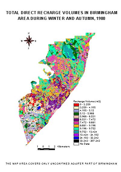
Figure 3. Recharge Distribution in Birmingham during autumn and winter 1980.

Nonpoint source (NPS) pollution is an exceedingly complex phenomenon. Nonpoint source pollution may be defined as the introduction of impurities into surface or sub-surface water supplies, generally from indirect, intermittent or diffuse sources and often associated with storm, rainfall or snowmelt events (Warrington, 2000). Nonpoint source pollution results from a wide variety of human activities on the land. It represents the cumulative effects of all of the land uses in a watershed and associated human activity. Owing to this complexity, models that try to reflect the actual processes require large quantities of data, which are rarely available. Thus, the most common method of approximating non-point source pollution uses long-term average contaminant loadings for common land uses. This approach is based on the National Urban Runoff Program called NURP (US EPA, 1984). The approach has been followed in many other countries also. The estimation of non point source pollutants in the surface runoff and recharge is based on typical Event Mean Concentrations. EMCs are standardized concentrations of a pollutant expected from a particular land use type. They are assumed to be directly related to the land uses in the watershed and remain constant independently of the duration and intensity of the rainfall events (Naranjo, 1998). Literature based Estimated Mean Concentrations of pollutant constituents associated with land use are available (Lopes and Dionne, 1998; Delzer et al., 1996 & Shepp, D.L., 1996).

In order to develop an NPS model dealing nitrate, chloride and BTEX compounds in runoff and infiltration and to predict actual concentration reaching to the water table, typical EMC values for the existing urban land uses have to be assigned. In Birmingham, very little study has been conducted on assessing detailed land use based storm water chemistry and pollutant loading estimation of the chosen pollutants. As a result, EMC data pertaining to all the possible urban land use classes in the Birmingham area not currently available. However, recent studies undertaken by Antonio, E. (1999) and Harris, (2000) do provide information on the concentrations of metals and inorganics, including values of nitrate and chloride, from specific land uses such as roads, car parks and lawn areas, observed within the Birmingham University campus.

Using the latter information together with other EMC data from literature, EMC values for six chosen constituents viz. nitrate, chloride, benzene, toluene, ethyl benzene, and xylene (Table 5) were identified to the modelling work of Birmingham. It may be noted that most of the EMC values in this table are compiled from many NPS case studies undertaken in US by EPA, USGS, USDA-NRCS and other organisations. The literature survey could not provide typical value for all the existing land uses in Birmingham. For some of the land use classes the typical EMC values had to be estimated based on the personal judgement depending on the land use type. Sometimes adequate EMC data were not available for a land use or contaminant, for example BTEX compounds. In these cases, estimates of EMCs were also made.

Using ArcView GIS, a model called ‘NPS pollutant load in runoff’ has been generated for estimating the pollutant loads of chosen constituents in surface runoff water (Fig.). The Avenue script written in this program/model associates or links EMC value of various pollutant constituents to the land use types. The input data for this model are: a) a grid of land uses in the urban area, b) a grid of average annual runoff volume in the basin and c) associated EMC values of chosen / selected pollutant constituents (nitrate, chloride, benzene, toluene, ethyl benzene, xylene and total suspended solids).

This program creates an EMC grid (for the above selected pollutants) and multiplies it by a grid of average annual rainfall runoff in the basin. The result will be the annual loading of the NPS constituent to each grid cell in the urban area, i.e.:

L (Mass/Time) = Q (Volume/Time) * C (Mass/Volume) (Equation 12)

The output from this model consists of predicted annual pollutant loading (e.g. mg/m²/year) for each land use type, which affects the urban watershed.

The typical pollutant concentration associated with various land use categories in the study area, i.e. EMC value, can be used for estimating the initial NPS pollutant fluxes in the infiltrated water also. Therefore, using this relationship, on multiplying the volume of infiltrated water with the EMC value would give an estimate of the initial pollutant fluxes in the recharge.

The infiltrated water is subject to evaporative loss across the soil-air interface and hence the concentration of the recharge water will be higher than that of the infiltrated water. The potential recharge value, calculated in the runoff-recharge model, is the quantity of infiltrated water left after the adjustment for loss through evaporation.

The calculated pollutant flux is the starting NPS pollutant fluxes, which enter the top part of the unsaturated zone, and is subject to the various physicochemical processes while it pass through the entire thickness of the unsaturated zone. The starting or initial NPS pollutant concentration in the recharge water can be estimated as:

Using the above relationships, (equations 12, 13 and 14) another sub model called "initial NPS recharge pollutant flux model" has been programmed in the ArcView GIS to estimate the initial pollutant flux and initial pollutant concentration in the recharge water. This model requires the following input data:

• Typical pollutant concentration value for each land use (EMC)
• Direct Runoff Volume grid map
• Cumulative infiltration volume grid map
• Potential recharge volume grid map

Figure 4. Interface of ArcView GIS based Nonpoint Source BTEX Pollution Model

The output from this sub-model is a series of maps showing the spatial distribution of initial pollutant fluxes and initial concentration in the recharge for the chosen parameters (nitrate, chloride and BTEX compounds). The concentrations of NPS pollutants and pollutants loads of the chosen constituents in the runoff water are also estimated while running this model.

Pollutants in the infiltrating recharge water may be subjected to various subsurface natural attenuation processes (such as sorption / retardation, in case of any volatile contaminant then vaporisation / volatilisation, and biodegradation, other transformation through microbiological activities etc) as it migrate though the vadose zone, whereas few pollutants like chloride in recharge remain as ‘non reactive’. Among the six pollutants chosen for GIS modelling under the present research, chloride is the only non-reactive solute; hence, the final concentration of chloride in the recharge can be modelled as equal to the initial concentration. The BTEX chemicals in the recharge are subject to sorption/desorption, biodegradation and volatilisation processes, whereas the nitrates are subject to other biological activities such as denitrification, uptake by the plants, nitrification and nitrogen fixation etc. Prediction of nitrate fate and leaching in the unsaturated zone is difficult due to the complex nature of the processes dominating the fate of nitrogen in soils. It was for this reason that it was decided to consider nitrate as a 'non-reactive' solute during its vadose zone migration. Thus, the initial concentration predicted (Figure 5) in the previous model is treated as the concentration entering to the water table.

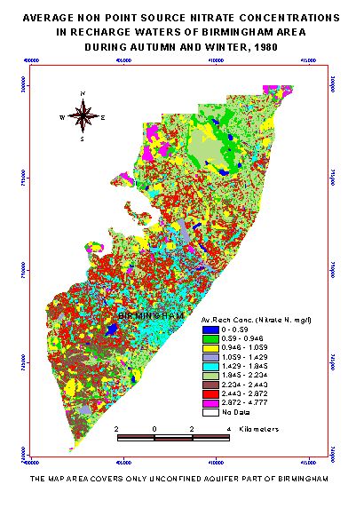
Figure 5. Nonpoint source nitrate (as N) concentration in the recharge.

In this model, the BTEX recharge pollutant fluxes are estimated through four stages viz.:

1. Estimation of volumetric water content in the unsaturated zone (using Clapp and Hornberger method)
2. Calculation of soil-water partitioning coefficients, K_d
3. Calculation of unsaturated zone retardation factor for BTEX compounds
4. Calculation of final BTEX concentration and BTEX pollutant mass flux entering to the water table.

The volumetric water content in the vadose zone can be calculated using the Clapp and Hornberger method (Clapp and Hornberger, 1978). Using Clapp and Hornberger method the volumetric water content of soil, q _w is given by

where q s is the saturated water content of the soil (total porosity)

V_d is the recharge rate

k_s is the saturated hydraulic conductivity at the saturated water content q s

b is the Clapp and Hornberger constant for the soil.

This is the constant in the Clapp and Hornberger equation relating the relative saturation of the soil to the relative conductivity of the soil (Clapp and Hornberger, 1978).

where k is the hydraulic conductivity of the soil at a volumetric water content q and k_s is the saturated hydraulic conductivity at the saturated water content q _s (total porosity in fraction). b is Clapp and Hornberger constant. If b is not known it can be estimated using the values presented by Clapp and Hornberger for different soil textures (Clapp and Hornberger, 1978).

The required input data for this sub-model are soil texture type, porosity, saturated hydraulic conductivity and Clapp and Hornberger constant values for the respective soil texture present. The various sub programs/codes provided in this model (Figure 4) help in assigning input data and later calculate the volumetric water content.

Soil-water partitioning coefficient, K_d, (also called soil adsorption coefficient or soil water sorption coefficient, Ks), expresses the tendency of a chemical compound to be adsorbed onto soil or rock or sediment particles. Over time, the dissolved contaminant will migrate from the free water and sorb onto soil or rock particles by a process called sorption. Sorption is an important process affecting the transport of contaminants in the subsurface. Due to sorption the leading edge of dissolved chemical plume moves slower than the infiltrating recharge water flow and or the groundwater flow, thus the contaminant migration rate or velocity is retarded, which is called retardation. The magnitude of the sorption for most soil water system is dependant on the hydrophobicity (measured by aqueous solubility) of the chemical and organic carbon content of the soil (Gustafson et al., 1997).

At equilibrium, a non-polar organic compound is seen to distribute itself between aqueous concentration C_w and sorbed concentration C_s, as a function of their ratio: K_d = C_s /C_w, with K_d the soil sorption or partition coefficient. The slope of the line plotting the liquid phase (aqueous) concentration versus the solid phase (sorbed) concentration for various combinations of liquid phase and solid mass concentrations is K_d. The value of K_d for a given organic compound is not constant, however, but researchers (Karickhoff et al., 1979) have found that for non-ionic hydrophobic chemicals the primary soil property controlling sorption is the fraction of organic carbon content of the soil. It has been that the value of K_d tends to increase linearly for soils with increasing organic carbon and clay contents. The slope of the relationship between K_d and % organic carbon is the amount of sorption on a unit carbon content basis called K_oc (Hassett and Banwart 1989), in which K_oc = K_d /f_oc where f_oc is the fraction of organic content in the soil.

Therefore, the soil-water partitioning coefficient, K_d can be estimated using the following relation/equation

K_d = K_oc f_oc

where K_d = soil-water partitioning coefficient

This sub-model simulates the downward movement of pollutant with soil solution and estimates the concentration of pollutants and pollutant flux from the vadose zone.

In a steady state single-phase flow system the average linear ground water velocity, v_i, is given as

where q is flux of ground water in steady state single phase flow;

n is porosity of the medium.

In the unsaturated zone, the term q can be replaced by the recharge flux and porosity can be replaced by the volumetric water content, q . Therefore, the velocity of the pollutant in the vadose zone is given by

V_p = V_a / R_f

where V_a = Aqueous or pore water velocity;

R_f = Retardation factor for the pollutant in the vadose zone.

Recharge rate V_d is the average downward flux density of water through the vadose zone (expressed as m / day).

Or in other form the velocity of the pollutant in the vadose zone can be calculated as

The retardation factor, R_f, for the vadose zone is calculated using the following equation:

R_f = 1 + (r K_d + (q _s - q ) K_H) / q

where r is the bulk density of the soil,

q _s is the saturated water content of the soil on a volume basis

K_d is the partition coefficient for pollutant in the soil

K_H is the dimensionless value of Henry’s law constant, (c_a /c_w).

The partition coefficient K_d can be calculated as K_ocf_oc where K_oc is the organic carbon partition coefficient and foc is the fractional organic carbon content of the soil. On comparing the above equation to the normal retardation equation for a saturated situation, R_f = 1 + (r K_d / q ) which does not contain any air phase, the difference noticed in it is the incorporation of Henry's law. The incorporation of Henry's law in the above equation helps to account for the loss of dissolved volatile organic compounds like BTEX through volatilisation. However, it has been noted that if volumetric water content is too low the use of the above equation might lead to the prediction of higher retardation factors.

The leading edge of the contaminated pulse will reach the water table at a time T that can be calculated as:

where z = depth of the vadose zone;

q = net recharge rate

In subsurface environments, biodegradation is known to reduce the level of contamination. Biodegradation is a natural process by which naturally occurring microorganisms such as bacteria, fungi breakdown soil and groundwater contaminants into less toxic substances. It can take place in the presence of oxygen (aerobic condition) or without oxygen (aerobic condition). In an aerobic environment, biodegradation of fuels generally follows a first order relationship. In addition, Salanitro (1993) has pointed out that biodegradation in laboratory microcosm experiments follows the first order reaction rule for aromatic hydrocarbons, including BTEX. Therefore, concentration of BTEX pollutants exiting the vadose zone can be estimated using the following first order decay model equation

C₂ = C₁ exp ^(-Tk)

where

T = percolation time or travel time through the vadose zone

where T_1/2 is the half life period; g = first order degradation rate coefficient for the chemical. Half-life period is the time required for getting one half of the original contaminant degraded. Substituting the travel time and degradation rate in the above equation, it becomes

This is the final equation programmed within the GIS to calculate final concentration reaching to the water table.

The one dimensional pollutant mass flux due to advection is equal to the quantity of the water flowing / infiltrating (net recharge rate) times the concentration of dissolved solids or solutes. Therefore, the BTEX pollutant loading / flux to the water table from the vadose zone is given as

or Flux = qC₂

i.e.,

The spatial distribution of the final pollutant concentrations and pollutant fluxes of Toluene in the recharge resulting from an average recharge rate simulation is shown in figure 6. It is interesting to note that nonpoint source pollution of BTEX in recharge waters is a problem only in areas having very shallow water table depths (especially near and/or on either sides of Tame river) whereas in rest of the area the model indicates that it is totally biodegraded.

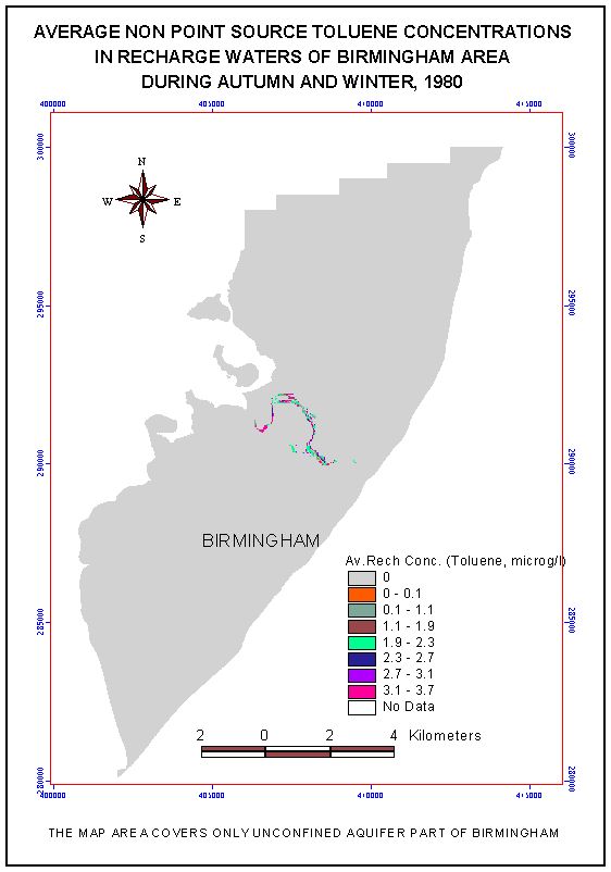
Figure 6. Nonpoint source toluene concentration in the recharge.

Little data exists pertaining to EMC values for Birmingham urban area characterised by a wide variety of land uses classes such as open green areas in many forms, residential, commercial / business, and heavy industrial. The published EMC values are often from studies in different climatic and hydrologic systems; therefore, site-specific sampling data should be used when it is available. The final pollutant concentrations and pollutant fluxes predicted in this model used EMC values based on national average estimates in United States. Their accuracy when applied to the Birmingham model will require further considerations but until further data becomes available these values represents the best estimates.

All units of the same land use type are assumed to have the same EMC value regardless of their spatial location within the city. However, in reality the concentration of pollutants in recharging water will vary depending on the soil type/vadose zone chemistry. From the made ground/drift/solid geology formations, release of the pollution to the recharge is possible due to past human activities e.g. accumulation of waste material. Sometimes the background concentration in the subsurface may add to the recharge. At present, this variability is not accounted in the model due to lack of information on the background chemistry and heterogeneity of the system.

The model is an experimental tool that has been applied to an urban area which is typical of many others that exhibit a high level of spatial heterogeneity and temporal variation resulting from both the natural and anthropogenic influences upon the ground and subsurface properties. In such a system it is often difficult to derive sensible data sets against which to test and calibrate such a model as this. Recharge may be directly measured but the data will be site specific and therefore difficult to relate to the larger scale. No such measurements are available for this study area though previous studies have estimated recharge using a numerical approach. The study by Greswell (1991) derived recharge estimates based on modelling of the groundwater flow system. The total recharge estimate from this model and that of Greswell are in close agreement.

The distributed contaminant fluxes from the GIS model will be input to a 3D groundwater flow model of the Birmingham aquifer that is currently under development. This will be used to identify areas of the unconfined aquifer that are most under threat from groundwater contamination resulting from pollutant sources. Conversely, areas relatively free of contamination (such as would be expected where the land use has predominantly been for residential dwelling or agricultural land) may be identified as potential areas of abstraction of higher quality water.

Estimation of recharge pollutant fluxes in urban environments is a complex spatial environmental problem. GIS is an appropriate tool for such environmental analysis. Clearly it will not be possible to develop a definitive representation of urban recharge and groundwater pollution processes, but it should be possible to set up a framework which, if the results are encouraging, will allow investigation of the main issues and which will be appropriate for progressive upgrading in future studies. This study will provide valuable information on the quality and quantity of groundwater and the risks of its use on a sustainable basis on a regional scale.

Authors would like to thank Commonwealth Scholarships Commission, United Kingdom, Natural Environment and Research Council, and Punjab Remote Sensing Centre, Ludhiana, India for financial and organisational support, which made this project possible.

Antonio, E. 1999. Stormwater Drain Chemistry and its Sources on the University of Birmingham Main Campus. Urban Regeneration and Environment (URGENT) Project, School of Earth Sciences, University of Birmingham.

Clapp, Roger B. and George M. Hornberger. 1978. Empirical equations for some soil hydraulic properties. Water Resources Research 14: 601-604.

Delzer-Gregory-C, Zogorski-John-S, Lopes-Thomas-J, and Bosshart-Robin-L. 1996. Occurrence of the gasoline oxygenate MTBE and BTEX compounds in urban stormwater in the United States, 1991-95. Water-Resources Investigations - U. S. Geological Survey.

http://sd.water.usgs.gov/nawqa/pubs/wrir/wrir96.4145/wrir.doc.html

EPA, 1998a. Estimation of Infiltration Rate in the Vadose Zone: Compilation of Simple Mathematical Models. Volume I. EPA/600/R-87/128a, February 1998. United States Environmental Protection Agency.

EPA, 1998b. Estimation of Infiltration Rate in the Vadose Zone: Application of Selected Mathematical Models. Volume II. EPA/600/R-87/128b, February 1998. United States Environmental Protection Agency.

Greswell, R.B., Lloyd, J.W., Lerner, D.N., and Knipe, C.V. (1994). Rising groundwater in the Birmingham area. WB Wilkinson (ed.), Groundwater problems in urban areas, Proc. Conf. Institution. Of Civil Engineers, June 1993,64-75, discussion 355-368.

Harris, J. 2000. Urban recharge from non-industrial areas in Birmingham. M.Phil. Research Project.

School of Earth Sciences, University of Birmingham, United Kingdom.

Johnson, Pool & Bloomer, 1991. Rising Groundwater Levels in Birmingham and the Engineering Implications. CIRIA Research Project RP 430. Johnson, Pool and Bloomer, and The School of Earth Sciences, University of Birmingham.

Karickhoff, S.N., Brown, D.S. and Scott, T.A. 1877. Sorption of hydrophobic pollutants in natural sediments. Water Research 13: 241- 248.

Lerner, D.N. (1997). Too much or too little: Recharge in urban areas. Groundwater in the urban environment, Vol. 1: Problems, Processes and Management, P.J. Chilton et al (eds.). Balkema, Rotterdam.pp 41-47.

Lerner, D.N. and Barrett, M.H., (1996). Urban Groundwater issues in the United Kingdom. Hydrogeology Journal, 4 (1) 80-89.

Lerner, D.N., Issac, A.S. and Simmers, I. (1990). Groundwater Recharge: A guide to understanding and estiamting natural recharge. International contributions to Hydrogeology, Volume 8, IAH. Hannover: Verlag Heinz Heise.

Lopes, T.J. and Dionne, S.G. 1998. A Review of Semivolatile and Volatile Organic Compounds in Highway Runoff and Urban Stormwater. U.S. Department of the Interior U.S. Geological Survey Open-File Report 98-409.

Naranjo, Eugenia. 1998. A GIS based nonpoint pollution simulation model. VKI, Institute for the Water Environment. Denmark.

http://proceedings.Esri.com/library/userconf/europroc97/4environment/E2/e2.htm

Salinitro, J.P. 1993. The role of bioattenuation in the management of aromatic hydrocarbon plumes in aquifers. Ground Water Monitoring Review. - Dublin, OH : Ground Water Publishing Co. Volume 13, 4/FALL, pp. 150-161.

Shepp, D.L. 1996. Petroleum Hydrocarbon Concentrations Observed in Runoff From Discrete, Urbanized Automotive-Intensive Land Uses. Metropolitan Washington Council of Governments, Washington, DC.

http://www.epa.gov/OWOW/watershed/Proceed/shepp.html

Tindall, James A., and Kunkel, James R. 1999. Unsaturated Zone Hydrology for Scientists and Engineers. Prentice-Hall, Inc.

USDA, 1986. Urban Hydrology for Small Watersheds. Technical Release-55. Natural Resources Conservation Service. United States Department of Agriculture.

Warrington, P. 2000. Best Management Practices to Protect Water Quality from Non-Point Source Pollution. March 2000. http://www.nalms.org/bclss/bmphome.html#nps

Yang, Y., Barrett, M.H. and Lerner, D.N.(1997). Assessing the impact of Nottingham on groundwater using GIS. Groundwater in the urban environment, IAH XXVII Congress, Nottingham.

Corresponding author: Abraham Thomas, Research Student, School of Earth Sciences, University of Birmingham, Edgbaston, Birmingham B15 2TT.United Kingdom. Telephone: *44 (0) 121 414 6146;

Fax: *44 (0) 121 414 4942; Email: a.thomas.1@bham.ac.uk.